tl;dr: the driving force of generative models
Modeling data distributions is a challenging and non-trivial task for high-dimensional and complex data such as images. Consider, for example, a simple \( 64 \times 64 \) RGB images with 8-bit color depth. Such an image contains $64\times64\times3=12,288$ dimensions, where each dimension can take one of 256 possible values. This results in a total of \( 256^{12288} \) possible configurations, an astronomically large space. Directly modeling such a distribution is therefore computationally infeasible. In this chapter, we discuss latent-variable modeling, where the objective is to capture the simpler, hidden variables that orchestrate the structure of the complex image data.
An unified framework
Observable phenomena often arise from simpler underlying structures. A complex signal, for example, decomposes into a sum of sinusoidal Fourier components, and a high-dimensional image reduces to a handful of principal components, or latent factors, that capture its essential variation. Generative modeling seeks to learn these latents with variable $\mathbf{z}\sim P_\mathbf{Z}$, to efficiently model data distributions. Let us refer to the transformation from data to latent as the forward process, since it increases entropy by progressively removing information. Conversely, the transformation from noise back to data is the reverse process. We can use the Bayes theorem to relate these processes as
\begin{equation}\label{eq:lvm} \underbrace{p(\mathbf{x} \mid \mathbf{z})}_{\text{reverse}} = \frac{\overbrace{p(\mathbf{z} \mid \mathbf{x})}^{\text{forward}} \, p(\mathbf{x})}{p(\mathbf{z})}. \end{equation}Hence, instead of modeling $P_\mathbf{X}$ directly, we can model its relationship with a much simpler, fixed latent distribution $P_\mathbf{Z}$ and use integration or sampling to obtain the complex distribution $P_\mathbf{X}$ as
\begin{equation} p(\mathbf{x})=\int p(\mathbf{x}\mid\mathbf{z})\,p(\mathbf{z}) \,\mathrm{d}\mathbf{z} \approx \mathbb{E}_{p(\mathbf{z})}[\,p(\mathbf{x}\mid\mathbf{z})\,] \end{equation}This enables both data generation (sampling novel instances from $\mathbf{z}$) and density estimation (computing likelihoods of $\mathbf{x}$ given $\mathbf{z}$), which constitute the fundamental objectives of generative modeling.
Latent Variable Models (LVMs) employ the forward and reverse transformations, also known as auto-encoding. We can intuitively understand how this works by considering language. Individual sounds lack meaning until humans structure them into complex sequences encoding thoughts and emotions. When we speak (encoding), listeners interpret our words (decoding), which is an imperfect process shaped by our subjective word choices. Yet, we can verify interpretation through sensory feedback. Hearing “tez!”1 when served dinner means little initially, but the sensation of a burning tongue makes the meaning unmistakably clear.
Where humans use language to make sense of our inner thoughts, generative models use mathematics as the language through which they make sense of data. Concretely, LVMs encode observed data to extract latent representations (analogous to speaking), decode latents to reconstruct data (analogous to listening), and verify consistency between original and reconstructed data. This process discovers meaningful latent structure that captures the essence of data.
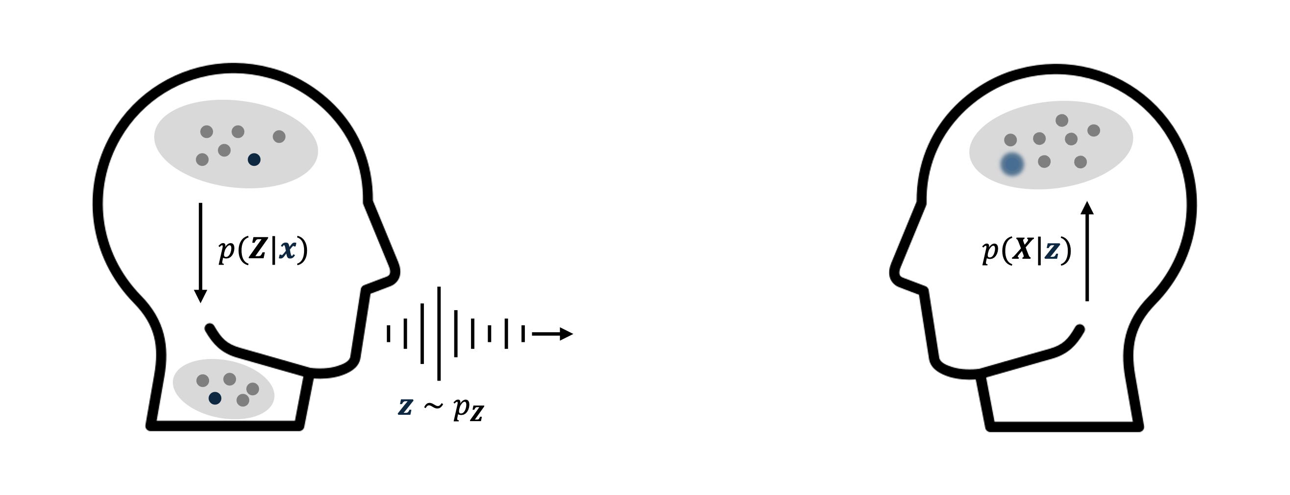
Generative modeling is often a form of auto-encoding, similar to learning a language.
In most frameworks, the latent distributions are modeled with a zero-mean isotropic Gaussian (for good reasons). The following sections will show how generative models employ the forward-reverse relationship, including
- Normalizing Flows learn a bijective forward process, which enables evaluating the reverse process using exact likelihoods of the model distribution.
- Generative Adversarial Networks directly model the reverse process originating from a lower-dimensional latent space.
- Variational Autoencoders model both the reverse and forward process subject to a compressed latent space.
- Denoising Diffusion Probabilistic Models learn the reverse process subject to a predefined forward process.
Normalizing Flows
Normalizing Flows provides a framework for generative modeling with exact likelihoods by constraining the transformation between latent and data space to be bijective, enabling exact and tractable density estimation. Equation (\ref{eq:lvm}) indicates that given any mapping \( p(\mathbf{x} \mid \mathbf{z}) \), we can compute the likelihood of the data through the inverse mapping \( p(\mathbf{z} \mid \mathbf{x}) \). Therefore, it makes sense to model the reverse process through some bijective function \( f: \mathbb{R}^D \rightarrow \mathbb{R}^D \) such that we can always evaluate both directions with \( \mathbf{x} = f(\mathbf{z}) \) and \( \mathbf{z} = f^{-1}(\mathbf{x}) \). The question remains: how to evaluate \( \frac{p(\mathbf{x})}{p(\mathbf{z})} \)? Using the law of probability, it can be written that
\begin{equation} \int p(\mathbf{x})\, \mathrm{d}\mathbf{x} = \int p(\mathbf{z})\, \mathrm{d}\mathbf{z} \quad \Leftrightarrow \quad p(\mathbf{x}) = p(\mathbf{z}) \left| \frac{\mathrm{d}\mathbf{z}}{\mathrm{d}\mathbf{x}} \right|, \end{equation}where the derivative represents the Jacobian determinant (proof). Since \( \mathbf{z} = f^{-1}(\mathbf{x}) \), this is equivalent to
\begin{equation} p(\mathbf{x}) = p(\mathbf{z}) \left| \det \frac{\mathrm{d} f^{-1}(\mathbf{x})}{\mathrm{d} \mathbf{x}} \right|. \end{equation}Then, the derivative can be rewritten as
\begin{equation} \frac{\mathrm{d} f^{-1}(\mathbf{x})}{\mathrm{d} \mathbf{x}} = \frac{\mathrm{d} \mathbf{z}}{\mathrm{d} \mathbf{x}} = \left( \frac{\mathrm{d} \mathbf{x}}{\mathrm{d} \mathbf{z}} \right)^{-1} = \left( \frac{\mathrm{d} f(\mathbf{z})}{\mathrm{d} \mathbf{z}} \right)^{-1}. \end{equation}Using the identity \( \det(\mathbf{A}^{-1}) = \frac{1}{\det(\mathbf{A})} \), the equation becomes
\begin{equation} p(\mathbf{x}) = p(\mathbf{z}) \left| \det \frac{\mathrm{d} f^{-1}(\mathbf{x})}{\mathrm{d} \mathbf{x}} \right| = p(\mathbf{z}) \left| \det \frac{\mathrm{d} f(\mathbf{z})}{\mathrm{d} \mathbf{z}} \right|^{-1}. \end{equation}Finding a single invertible function that maps \( \mathbf{z} \rightarrow \mathbf{x} \) would require an extremely complex model, making it practically infeasible. Instead, we concatenate multiple functions \( f = f_K \circ f_{K-1} \circ \cdots \circ f_1 \), each being a simple invertible transformation with a cheap Jacobian determinant. Such functions are known as flows. Given \( \mathbf{z}_k = f_k(\mathbf{z}_{k-1}) \) and \( \mathbf{z}_{k-1} = f_k^{-1}(\mathbf{z}_k) \). We can write
\begin{equation} p(\mathbf{z}_k) = p(\mathbf{z}_{k-1}) \left| \det \frac{\mathrm{d} f_k(\mathbf{z}_{k-1})}{\mathrm{d} \mathbf{z}_{k-1}} \right|^{-1}. \end{equation}Therefore, training consists of maximizing the total log-likelihood
\begin{equation} \log p(\mathbf{x}) = \sum_{k=1}^K \log p(\mathbf{z}_k) - \sum_{k=1}^K \log \left| \det \frac{\mathrm{d} f_k(\mathbf{z}_{k-1})}{\mathrm{d} \mathbf{z}_{k-1}} \right|. \end{equation}Similarly, evaluation of a novel image pertains finding the corresponding $\mathbf{z}$ and its likelihood on $P_\mathbf{Z}$, while also determining the log-Jacobian determinant of each intermediate function $f_k^{-1}(\mathbf{z}_k)$.
Flow types
Ideally, a NF is sufficiently expressive within as little steps as possible, while having an easy inversion and calculation of the Jacobian determinant. For example, let $\mathbf{A}\in\mathbb{R}^{D\times D}$ be an invertible matrix and $\mathbf{b}\in\mathbb{R}^D$ an arbitrary vector. The Linear Flow can be defined as
\begin{equation} f(\mathbf{x}):=\mathbf{A}\mathbf{x}+\mathbf{b}. \end{equation}Indeed, as $\mathbf{A}$ is invertible, we can find $\mathbf{A}^{-1}$. The Jacobian, $\det \mathbf{A}$, becomes expensive as the dimensionality of the data increases. Hence, some restrictions can be placed upon $\mathbf{A}$, such as it being triangular, orthogonal or factorizing it through LU decomposition. However, a Linear Flow cannot transform a density “out of its family”, i.e. an exponential density will stay exponential. More expressive flows include the Planar flow2, expands and contracts distributions along a direction, which can be defined as
\begin{equation} f(\mathbf{x}):= \mathbf{x} + \mathbf{u} \, h(\mathbf{w}^T\mathbf{x} + b), \end{equation}with parameters $\mathbf{u}, \mathbf{w} \in \mathbb{R}^D$ and $b \in \mathbb{R}$. The Jacobian determinant becomes (with use of the matrix determinant lemma)
\begin{equation} \det \frac{\mathrm{d} f}{\mathrm{d} \mathbf{x}} = \mathbf{1} + \frac{\mathrm{d} h}{\mathrm{d}\mathbf{x}} (\mathbf{w}^T\mathbf{x} + b)\,\mathbf{u}^T \mathbf{w}. \end{equation}However, these approaches remain less prevalent in image modeling than coupling flows, particularly affine coupling layers, which are central to RealNVP3 and later Glow4. A key computational advantage of this architecture is that the scale and translation functions can be arbitrarily complex neural networks without complicating the flow’s inverse or the Jacobian determinant calculation, which remains triangular and efficient (more details).
Dequantization
Training a continuous density model directly on discrete data yields degenerate solutions, in which the model places ever-increasing density on individual data points rather than learning a smooth distribution. To resolve this, a technique known as dequantization can be employed. This involves adding noise, sampled from a specific distribution $q(\mathbf{u}\mid \mathbf{x})$ with continuous support over $\mathbf{u}\in [0,1)$ to create dequantized variables $\tilde{\mathbf{x}}=\mathbf{x}+\mathbf{u}$ as
\begin{equation}\label{eq:dequant} p_{\mathbf{X}}= \int p_{\mathbf{X}} (\mathbf{x}+\mathbf{u})\mathrm{d}\mathbf{u} = \int \frac{q(\mathbf{u}\mid\mathbf{x})}{q(\mathbf{u}\mid\mathbf{x})} p_{\mathbf{X}}(\mathbf{x}+\mathbf{u})\mathrm{d}\mathbf{u} \approx \mathbb{E}_{q(\mathbf{u}\mid\mathbf{x})} \left[ \frac{p_{\mathbf{X}}(\mathbf{x}+\mathbf{u})}{q(\mathbf{u}\mid\mathbf{x})}\right]. \end{equation}Thus, integer $\mathbf{x}=0$ becomes a continuous variable $\tilde{\mathbf{x}}\in [0.0, 1.0)$, $\mathbf{x}=1$ becomes $\tilde{\mathbf{x}}\in [1.0, 2.0)$ etc. The noise distribution can be chosen to be uniform, which requires the model to learn sharp edges around the cubes $\mathbf{x} +[0,1)$, which is a challenging tasks for neural networks. Hence, it is also possible to learn the noise distribution through a flow itself, where the forward process is defined as
\begin{equation} q(\mathbf{u}\mid\mathbf{x}) = p_{\mathbf{\epsilon}}(q_{\mathbf{X}}^{-1}(\mathbf{u})) \cdot \left| \frac{\partial q_{\mathbf{X}}^{-1}}{\partial \mathbf{u}} \right|, \end{equation}with $\mathbf{u}=q_{\mathbf{X}}(\mathbf{\epsilon})$ and $p_{\mathbf{\epsilon}}(\mathbf{\epsilon})=\mathcal{N}(\mathbf{\epsilon}; \mathbf{0}, \mathbf{I})$. As such, we can substitute this in Equation (\ref{eq:dequant}) to obtain the objective
\begin{equation} \mathbb{E}_{q(\mathbf{u}\mid\mathbf{x})} \left[ \log \frac{p_{\mathbf{X}}(\mathbf{x}+q_{\mathbf{X}}(\mathbf{\epsilon}))}{p(\mathbf{\epsilon}) \cdot \left\| \partial q_{\mathbf{X}} / \partial \mathbf{\epsilon} \right\|^{-1}}\right]. \end{equation}This leads to a better and smoother and representation of the data, which in turn can improves the learned model distribution. Jensen’s Inequality can be used to show that
\begin{equation} \begin{aligned} \mathbb{E}_{\tilde{\mathbf{x}}\sim P_{\tilde{\mathbf{X}}}} [\log p_{\tilde{\mathbf{X}}}(\tilde{\mathbf{x}})] &= \sum_{\mathbf{x}} P_{\mathbf{X}}(\mathbf{x}) \int \log \frac{p_{\mathbf{X}}(\mathbf{x}+\mathbf{u})}{q(\mathbf{u}\mid\mathbf{x})} q(\mathbf{u}\mid\mathbf{x}) \mathrm{d}\mathbf{u} \\ &\leq \sum_{\mathbf{x}} P_{\mathbf{X}}(\mathbf{x}) \log \int \frac{p_{\mathbf{X}}(\mathbf{x}+\mathbf{u})}{q(\mathbf{u}\mid\mathbf{x})} q(\mathbf{u}\mid\mathbf{x}) \mathrm{d}\mathbf{u} \\ &= \mathbb{E}_{\mathbf{x}\sim P_{\mathbf{X}}} [\log p_{\mathbf{X}}(\mathbf{x})], \end{aligned} \end{equation}meaning the continuous model subject to dequantized data $\tilde{\mathbf{x}}$ will never collapse to a particular one on the discrete data because it is bounded from above by the degenerate model trained on discrete data $\mathbf{x}$.
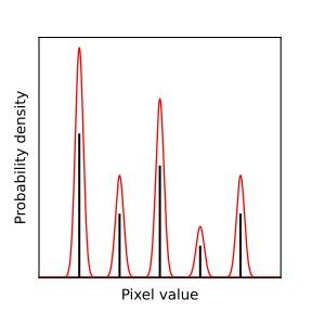
No dequantization
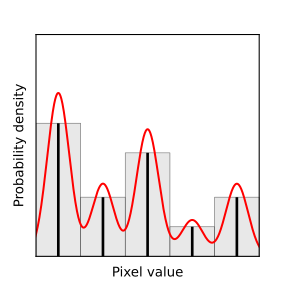
Uniform dequantization
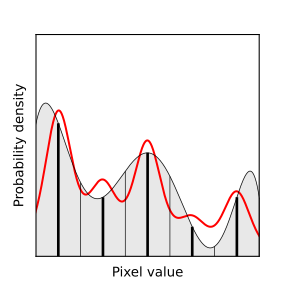
Variational dequantization
Generative Adversarial Networks
So far, we have examined generative modeling primarily through the lens of likelihood functions. In some settings, however, explicit likelihood estimation is unnecessary. When the goal is simply to generate realistic samples resembling the target data distribution, one can directly learn the mapping $P_{\mathbf{X}\mid\mathbf{Z}}$ through generative matching. Because exact likelihood estimation is out-of-scope, we can reduce the dimensionality of $\mathbf{z}$ to values smaller than $\mathbb{R}^D$ and deploy the reverse process as
\begin{equation} p_{\mathbf{X}\mid\mathbf{Z}}=\mathcal{N}(\mathbf{\mu}=\text{G}_1(\mathbf{z}),\mathbf{\Sigma}=\text{G}_2(\mathbf{z})), \end{equation}where functions $\text{G}_1:\mathbb{R}^d\rightarrow\mathbb{R}^D$ and $\text{G}_2:\mathbb{R}^d\rightarrow\mathbb{R}^{D\times D}$ can be arbitrarily complex. A practical difficulty is that the covariance matrix scales with the square of the image dimensions. We therefore assume a diagonal covariance, treating the output pixels as mutually independent, and fix $\text{G}_2=\mathbf{\sigma}$ to a constant value. We can then write
\begin{equation}\label{eq:generativem1} p(\mathbf{x}\mid\mathbf{z}) = \frac{1}{\sqrt{2\pi}\cdot \mathbf{\sigma}^2}e^{-\frac{(\mathbf{x}-\text{G}_1(\mathbf{z}))^2}{2\cdot \mathbf{\sigma}^2}}. \end{equation}Taking the logarithm results in
\begin{equation} \log p(\mathbf{x}\mid\mathbf{z}) = - \frac{1}{2} \ln (2\pi \cdot \mathbf{\sigma}^2)-\frac{1}{2\cdot \mathbf{\sigma}^2}(\mathbf{x}-\text{G}(\mathbf{z}))^2 \approx -(\mathbf{X} - \text{G}(\mathbf{z}))^2, \end{equation}Note that this is identical to the Mean Squared Error objective up to a multiplicative constant. Goodfellow5 present the GAN, which introduced a secondary discriminative network $\text{D}:\mathbb{R}^D \rightarrow[0,1]$ to effectively serve as a competitor to $\text{G}$. To state in simple terms, generator $\text{G}$ attempts to produce images that realistically resemble the training set while discriminator $\text{D}$ attempts to correctly classify the generated images to either “real” or “fake/generated”, corresponding to images from the data and model distribution, respectively. The objective for both $\text{G}$ and $\text{D}$ can be phrased as
\begin{equation}\label{eq:ganobjective1} J (\boldsymbol{\theta}_\text{G}, \mathbf{\boldsymbol{\theta}}_\text{D}) = \mathbb{E}_{\mathbf{x}\sim P_\mathbf{X}} [\,\log \text{D}(\mathbf{x}) \,] + \mathbb{E}_{\mathbf{z}\sim p_\mathbf{Z}} [\, \log (1-\text{D}(\text{G}(\mathbf{z})))\,]. \end{equation}The term adversarial reflects the fact that two networks are trained in opposition to each other. In other contexts, adversarial samples are inputs crafted to “attack” a network and expose its weaknesses. Here, the adversarial setup instead pits the generator $\text{G}$, which tries to produce realistic images, against the discriminator $\text{D}$, which tries to distinguish real data from generated data.
The dynamic resembles that of a counterfeiter and a shopkeeper. The counterfeiter, $\text{G}$, wants to produce fake banknotes good enough to pass, while the shopkeeper, $\text{D}$, tries to tell real from fake. Crucially, the two must improve together. Without a shopkeeper, the counterfeiter gets no feedback on what gives the fakes away. If a shopkeeper is flawless from the start, he offers nothing to learn from since every note is simply rejected. Only when both improve gradually, each responding to the other, does the counterfeiter learn to produce convincing notes.
Game theoretic dynamics
Since the goal is to generate realistic images, $\text{G}$ should “win” after sufficient resistance from $\text{D}$. In other words, $\text{D}$ is not able to distinguish real from generated images of $\text{G}$ and outputs $\frac{1}{2}$ for all data.
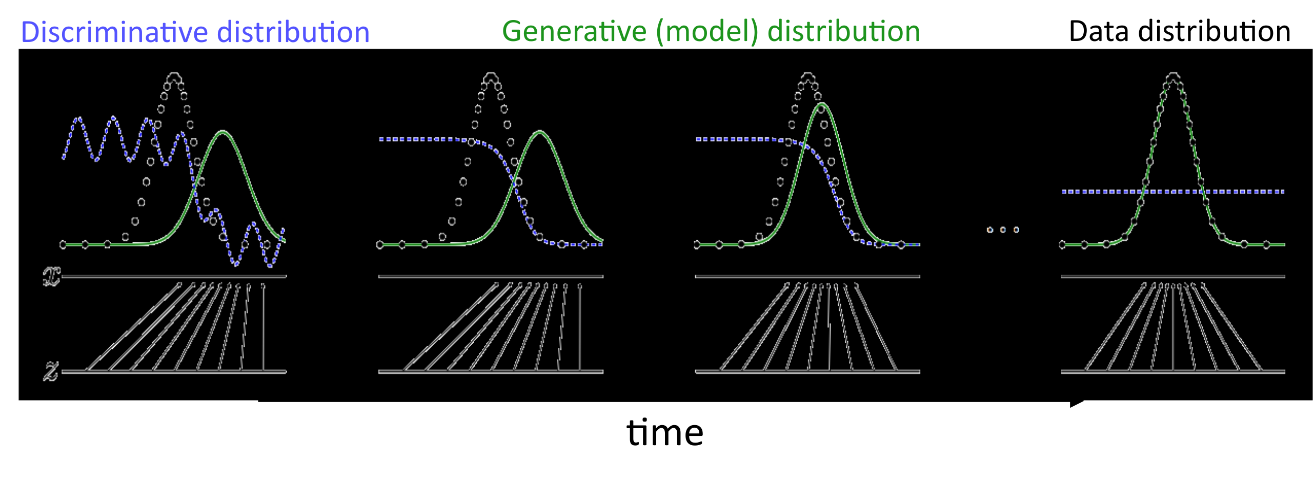
The generator should eventually converge to the optimal solution after sufficient resistance from the discriminator, adapted from7
Training essentially entails a mini-max game, where the generator minimizes an objective that the discriminator maximizes, representing the best outcome a player can guarantee itself when the opponent plays its worst-case response. Building on this game-theoretic view, a Nash equilibrium is reached when neither $\text{G}$ nor $\text{D}$ can gain by changing strategy, though simple examples show this equilibrium may be unattainable in practice. For example, imagine two players, one minimizing $\mathbf{x}$ and the other maximizing $\mathbf{y}$, with cost $J(\mathbf{x}, \mathbf{y}) = \mathbf{x} \cdot \mathbf{y}$. The gradient descent–ascent procedure can be written compactly as
\begin{equation} \mathbf{u}_{k+1} = \mathbf{u}_k + s_{\mathbf{u}} \, \eta \nabla_{\mathbf{u}} J(\mathbf{x}_k, \mathbf{y}_k), \qquad \mathbf{u} \in \{\mathbf{x}, \mathbf{y}\}, \end{equation}where $s_{\mathbf{x}} = -1$ (descent) and $s_{\mathbf{y}} = +1$ (ascent). Assuming time-continuous gradient updates with infinitesimal learning rate, we can write
\begin{equation} \frac{\partial \mathbf{u}}{\partial t} = \lim_{\eta \to 0} \frac{\mathbf{u}_{k+1} - \mathbf{u}_k}{\eta} = s_{\mathbf{u}} \nabla_{\mathbf{u}} J(\mathbf{x}(t), \mathbf{y}(t)), \qquad \mathbf{u} \in \{\mathbf{x}, \mathbf{y}\},\ \end{equation}such that
\begin{equation} \frac{\partial^2 \mathbf{y}}{\partial t^2}=\frac{\partial \mathbf{x}}{\partial t}=-\mathbf{y}(t). \end{equation}This differential equation has the solution of an infinitely long circular orbit and only admits an equilibrium when initialized at its optimal point. In practical gradient descent, however, the learning rate $\eta$ is not infinitesimal. For nonzero $\eta$, the discrete updates no longer follow the closed circular orbit but instead spiral outward, producing oscillations of progressively increasing amplitude. This divergent oscillatory behavior can translate into the unstable training of GANs.
Training issues
Although GANs were among the earliest models to demonstrate the potential of LVMs, their results were limited by training pathologies. For example, it is hard to gauge how well $\text{D}$ should perform relative to $\text{G}$, and the loss function gives little indication of progress. Also, a distinct failure mode is mode collapse. If $\text{D}$ initially struggles with particular image semantics, $\text{G}$ can exploit this by repeatedly producing those same features to minimize its loss, yielding biased and often unrealistic outputs. The precise causes of mode collapse remain poorly understood, and the literature does not agree on them.
Furthermore, when $P_\text{G}$ and $P_\mathbf{X}$ are non-overlapping, for instance when both lie on a lower-dimensional manifold or have disjoint supports, the gradients of $\text{G}$ can vanish, the so-called vanishing gradient problem. A common remedy is the alternative generator objective $\nabla_{\boldsymbol{\theta}_\text{G}} \mathbb{E}_{p_{\mathbf{Z}}} [-\log \text{D}(\text{G}(\mathbf{z}))]$, which empirically alleviates vanishing gradients and yields good samples. This fix, however, makes training highly unstable, producing weight updates with zero expected value but infinite variance6. The choice of generator cost therefore amounts to a trade-off between vanishing gradients and unstable training.
Because training GANs is so challenging, a substantial body of research is devoted to stabilizing it. Proposed remedies include structural guidelines for designing GAN architectures7; feature matching, which aligns the statistics of generated and real outputs8; minibatch discrimination, which feeds inter-sample relationships within a batch to $\text{D}$8; historical averaging, which penalizes deviations from past parameter values8; one-sided label smoothing, which softens the real labels to $1-\epsilon$8; virtual batch normalization, which normalizes each batch against a fixed reference batch8; the addition of correlated noise to broaden the support of $P_{\mathbf{X}}$6; and alternative cost functions such as the Wasserstein metric9.
Variational Autoencoders
In this section, we explore a seemingly middle ground between NFs and GANs. VAEs learn both a lower-dimensional latent representation while retaining a likelihood-based training objective. The name variational comes from the fact that the true encoder is approximated with a simpler family of posteriors. Specifically, we approximate the Bayesian posterior in Equation (\ref{eq:lvm}) with parameterized variational distribution \( q_{ \boldsymbol{\theta}}(\mathbf{z} \mid \mathbf{x}) \) and model $p_{ \boldsymbol{\phi}}(\mathbf{x})=\int p_{ \boldsymbol{\phi}} (\mathbf{x}\mid\mathbf{z}) p(\mathbf{z})\mathrm{d}\mathbf{z}$. With Jensen’s inequality we can find the lower bound
\begin{align} \log p_{ \boldsymbol{\phi}}(\mathbf{x}) &= \log \int q_{ \boldsymbol{\theta}}(\mathbf{z}\mid\mathbf{x})\frac{p_{ \boldsymbol{\phi}}(\mathbf{x},\mathbf{z})}{q_{ \boldsymbol{\theta}} (\mathbf{z}\mid\mathbf{x})}\mathrm{d}\mathbf{z} \geq \int q_{ \boldsymbol{\theta}}(\mathbf{z}\mid\mathbf{x}) \log\frac{p_{ \boldsymbol{\phi}}(\mathbf{x},\mathbf{z})}{ q_{ \boldsymbol{\theta}}(\mathbf{z}\mid\mathbf{x})}\mathrm{d}\mathbf{z} \notag \\ &= \underbrace{\mathbb{E}_{q_{ \boldsymbol{\theta}} (\mathbf{z}\mid\mathbf{x})} [\,\log p_\phi (\mathbf{x}\mid\mathbf{z}) \,]}_{\text{reconstruction}} - \underbrace{\operatorname{KL}[\,q_\theta (\mathbf{z}\mid\mathbf{x})\,\mid\mid\,p(\mathbf{z})\,]}_{\text{prior matching}}.\label{eq:celbo} \end{align}This is known as the Evidence Lower Bound (ELBO). The first term indicates how good the decoded data resembles the original input of the approximate posterior. The second term ensures a specific structure of the posterior, which is set by choosing an appropriate prior $p(\mathbf{z})$. Because the approximate posteriors are regularized toward this prior, we expect them to match the prior distribution after training. Consequently, we can generate novel test samples by drawing from prior $\mathbf{z}\sim p_\mathbf{Z}$ and running it through the decoder $p_{\phi} (\mathbf{x}\mid\mathbf{z})$. Note that by learning a decoding, we are also implicitly learning the true, intractable, encoding since
\begin{equation} p_{ \boldsymbol{\phi}} (\mathbf{z}\mid\mathbf{x}) = \frac{p_\phi (\mathbf{x}\mid\mathbf{z})\, p(\mathbf{z})}{p(\mathbf{x})}. \end{equation}If the approximate posterior $q_\theta(\mathbf{z} \mid \mathbf{x})$ were equal to the true posterior $p_\phi(\mathbf{z} \mid \mathbf{x})$, the bound in Equation (\ref{eq:celbo}) would hold with equality. The slack is $\mathrm{KL}[\, q_\theta(\mathbf{z} \mid \mathbf{x}) \,\|\, p_\phi(\mathbf{z} \mid \mathbf{x}) \,]$, implying that maximizing the ELBO pressures the approximate posterior toward the true posterior of the generative model. Predicting these distributions with a single shared network rather than per datapoint amortizes the inference, at the cost of an additional error known as the amortization gap10. This type of inference error occurs alongside the approximation error, which results from the chosen variational distribution’s inability to model the true posterior.
Finally, the reparameterization trick11 recasts sampling as a differentiable transformation, allowing gradients to flow through the stochastic node. Noise is drawn as $ \mathbf{\epsilon}\sim \mathcal{N}( \mathbf{0}, \mathbf{I})$ and used to compute $\mathbf{z} = \boldsymbol{\mu} + \boldsymbol{\sigma} \cdot \boldsymbol{\epsilon}$, i.e., scaling the noise by the standard deviation and shifting by the mean. The mean $\boldsymbol{\mu}$ and standard deviation $\boldsymbol{\sigma}$ are now deterministic functions of the input, with the stochasticity confined to $\boldsymbol{\epsilon}$, so gradients can propagate through them.
Posterior collapse
High-dimensional observations are often assumed to lie on a low-dimensional manifold. By working with VAEs, we can both project the data into a lower-dimensional latent space and estimate a lower bound on the data log-likelihood. This formulation enables probabilistic interpolation in the latent space, allowing exploration and manipulation of data attributes. Nevertheless, training VAEs can often be hindered by significant challenges such as the inefficient utilization of latent variables, a phenomenon commonly referred to as posterior collapse12,13. In severe cases, the latent variables are effectively ignored, serving only as a source of stochasticity for sampling. This behavior causes the VAE to degenerate towards a GAN-like regime.
Why does posterior collapse occur? Research mainly addresses the variational objective as the culprit14,12,15,16,17,18,19. Chen et al.20 relate the VAE to the bits-back coding mechanism and argue that whenever there is a way to ignore $\mathbf{z}$, it will be ignored. Another line of reasoning attributes posterior collapse to an overly powerful decoder, with one common remedy being to reduce the capacity of the generative decoder21,12,22. Others argue that the amortization of the ELBO might be the culprit10. However, recent theoretical work suggests it to be an intrinsic issue with the ELBO objective23. Wang et al.24 show that posterior collapse occurs precisely when the data place no constraint on the latent variables, a property of the generative model rather than of the inference procedure. They demonstrate that it can therefore arise even in classical models under exact inference.
The main message is that a VAE may ignore its latent variables whenever doing so does not reduce its ability to model the data. This behavior can stem from the objective itself, not just from an overly expressive decoder or imperfect inference, as is often suggested. When using VAEs for representation learning, the latent variables must be meaningfully engaged and the resulting likelihood estimates well-calibrated. In practice, this typically requires careful choice of latent dimensionality and additional constraints or specialized training techniques.
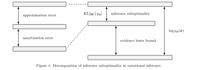
Improving Variational Inference
Collapse has been attributed to causes in the model, objective, inference, and architecture, with no firm consensus, and the proposed remedies intervene at correspondingly different levels. The most direct line of attack targets the decoder, on the intuition that a sufficiently powerful one can model the data while ignoring $\mathbf{z}$ entirely, so limiting its capacity forces reliance on the latent. This has been done by reducing its conditioning in text models12, removing fine-grained textural information in image models20, and limiting capacity through architectural choices such as dilated convolutions21.
Furthermore, the aggregate posterior must resemble the prior without matching it exactly, since an exact match is degenerate. A second group of methods therefore acts directly on the KL divergence, reweighting or monitoring it during training. Higgins et al.16 cast the VAE objective as a constrained optimization,
\begin{equation} \max_{ \boldsymbol{\theta}, \boldsymbol{\phi}} \; \mathbb{E}_{q_{ \boldsymbol{\theta}}(\mathbf{z}\mid\mathbf{x})}\!\left[\log p_{ \boldsymbol{\phi}}(\mathbf{x}\mid\mathbf{z})\right] \quad \text{s.t.} \quad \operatorname{KL}\!\left[ q_{ \boldsymbol{\theta}}(\mathbf{z}\mid\mathbf{x}) \,\parallel\, p(\mathbf{z}) \right] \le \delta, \end{equation}whose Karush–Kuhn–Tucker conditions yield the $\beta$-VAE objective
\begin{equation} \mathcal{L}_\beta( \boldsymbol{\theta}, \boldsymbol{\phi}) = \mathbb{E}_{q_{ \boldsymbol{\theta}}(\mathbf{z}\mid\mathbf{x})}\!\left[\log p_{ \boldsymbol{\phi}}(\mathbf{x}\mid\mathbf{z})\right] - \beta\,\operatorname{KL}\!\left[q_{ \boldsymbol{\theta}}(\mathbf{z}\mid\mathbf{x}) \parallel p(\mathbf{z})\right], \end{equation}with $\beta$ weighting the KL term. Setting $\beta>1$ encourages disentangled representations and is naturally read as a rate–distortion trade-off, where larger $\beta$ lowers the rate by allowing less information in the latent, at the cost of reconstruction quality, and smaller $\beta$ does the reverse. Related schemes reweigh the KL term through annealing schedules12,25, adversarial objectives26,27, or auxiliary decoders28. A related thread targets the mutual information between data and latents directly, replacing it with a proxy objective29, monitoring it as a stopping criterion30, or raising it via latent-to-data skip connections31.
Finally, a third group addresses collapse closer to its source by restructuring the latent representation itself or improving how it is inferred. Encoders have been extended to hierarchical, multi-level latents32,18 and to discrete codes, most notably VQ-VAE33. Other work lets groups of encoders compete to specialize in different latent concepts34, introduces a two-stage VAE for when the latent dimensionality exceeds the data manifold23, partially amortizes the inference19, or uses a DCT-based transform to select informative top-level latents35. A further line learns more flexible priors33,36,20,37 and more expressive posteriors38, for instance by augmenting the posterior with an NF2.
Denoising Diffusion Probabilistic Models
In this section, we take a relatively more explicit route of learning the data distribution. Rather than learning a mapping to latent space, the forward path is fixed from data to noise by hand and only the reverse process is learned. The derivations and explanations in this section are based upon the work of Luo et al.39, where we take the perspective of extending the ELBO to its hierarchical variant. See full derivation here. First, the latent dimensionality is set equal to that of the data, which removes the redundant notation of using $\mathbf{z}$ for the intermediate variables. Instead, all involved variables are denoted as $\mathbf{x}_t$, where $\mathbf{x}_0$ is the starting input image and $\mathbf{x}_T$ the variable deepest in the hierarchy. Furthermore, we assume a Markov process for all intermediate densities. Meaning each variable only depends on the previous as
\begin{equation} p (\mathbf{x}_{0:T}) = p(\mathbf{x}_T) \prod^T_{t=1} p (\mathbf{x}_{t-1} \mid \mathbf{x}_{t}). \end{equation}In this case, the ELBO can be written as
\begin{equation}\label{eq:ddpmelbo} \begin{aligned} \log p(\mathbf{x}) \geq \mathbb{E}_{q(\mathbf{x}_1\mid \mathbf{x}_0)} [\log p_\phi (\mathbf{x}_0 \mid \mathbf{x}_1)] - D_{KL} [ q(\mathbf{x}_T\mid\mathbf{x}_0)\mid\mid p(\mathbf{x}_T)] \\ \hspace{25pt}- \sum_{t=2}^T \mathbb{E}_{q(\mathbf{x}_t\mid \mathbf{x}_0)} \left[ D_{KL} [q (\mathbf{x}_{t-1}\mid\mathbf{x}_t, \mathbf{x}_0) \mid\mid p_\phi (\mathbf{x}_{t-1}\mid\mathbf{x}_t)]\right]. \end{aligned} \end{equation}As can be seen, this leaves us with three terms in the ELBO objective. The first term is regarding the likelihood of the original input image $\mathbf{x}_0$ given the previous timestep $\mathbf{x}_1$, reflecting the reconstruction cost. The second term ensures regularization such that the encoded variable $\mathbf{x}_T$ is distributed as the prior. Finally, the denoise matching terms ensure that the predicted noisy image from the learned reverse process resembles the ground truth. The crucial difference with this objective is that we will not learn the forward process, but design it ourselves, and learn the reverse process. We will begin by fixing the forward process to the linear Gaussian model
\begin{equation} q(\mathbf{x}_t\mid\mathbf{x}_{t-1}, \mathbf{x}_0) = \mathcal{N}(\mathbf{x}_t; \boldsymbol{\mu}=\sqrt{\alpha_t}\mathbf{x}_{t-1}, \boldsymbol{\Sigma}=(1-\alpha_t)\cdot\mathbf{I}), \end{equation}with mixing parameters $\boldsymbol{\alpha} = \{\alpha_t\}^T_{t=1}$, which control the diffusion process and ensure that the variances of $\mathbf{x}_t$ are retained. Usually the $\alpha_t$ schedule varies linearly with depth, but any monotone or even learned schedule is possible. Note that with this forward process, we can assume that $\mathbf{x}_T$ is distributed as $p_{\mathbf{Z}}$ without explicitly minimizing a KL-divergence, which enables us to effectively assume the first KL-divergence in Equation (\ref{eq:ddpmelbo}) to be zero. Finally, the number of steps $T$ is chosen large enough such that we can maximize the mutual information between sequential steps to ease learning the reverse process.
Parameterizing the reverse process
Having defined the forward process, we now reverse it: given $\mathbf{x}_t$ and $t$, what is $\mathbf{x}_{t-1}$? The true reverse posterior is Gaussian,
\begin{equation} q(\mathbf{x}_{t-1}\mid\mathbf{x}_t, \mathbf{x}_0) = \mathcal{N}\!\big(\mathbf{x}_{t-1}; \mu(\mathbf{x}_t, \mathbf{x}_0),\, \sigma^2(t)\,\mathbf{I}\big), \end{equation}with
\begin{align} \mu(\mathbf{x}_t,\mathbf{x}_0) &= \frac{\sqrt{\alpha_t}(1-\overline{\alpha}_{t-1})\mathbf{x}_t + \sqrt{\overline{\alpha}_{t-1}}(1-\alpha_t)\mathbf{x}_0}{1-\overline{\alpha}_t}, \label{subeq:forwardmean}\\ \sigma^2(t) &= \frac{(1-\alpha_t)(1-\overline{\alpha}_{t-1})}{1-\overline{\alpha}_t}. \label{subeq:forwardmvar} \end{align}We therefore model the reverse step as $p_\phi(\mathbf{x}_{t-1}\mid\mathbf{x}_t)=\mathcal{N}(\mathbf{x}_{t-1}; \mu_\phi(\mathbf{x}_t,t), \sigma^2_\phi(t)\,\mathbf{I})$ and, fixing $\sigma^2_\phi(t)=\sigma^2(t)$, fit $\mu_\phi$ to \eqref{subeq:forwardmean}. Matching the two Gaussians reduces the per-step objective to a weighted squared error between $\mu_\phi$ and $\mu$; the three standard parameterizations differ only in what the network predicts.
Predicting $\mathbf{x}_0$. Since $\mathbf{x}_0$ is the only unknown in \eqref{subeq:forwardmean}, the network can predict it directly, giving
\begin{equation} \arg \min_\phi D_{\text{KL}} = \arg \min_\phi \frac{1}{2\sigma^2(t)} \,\big\| \mathbf{x}_\phi(\mathbf{x}_t, t) - \mathbf{x}_0 \big\|^2_2 . \end{equation}Predicting the noise $\boldsymbol{\epsilon}_0$. Using the forward marginal $\mathbf{x}_t = \sqrt{\overline{\alpha}_t}\,\mathbf{x}_0 + \sqrt{1-\overline{\alpha}_t}\,\boldsymbol{\epsilon}_0$ to substitute for $\mathbf{x}_0$ rewrites the mean as
\begin{equation} \mu(\mathbf{x}_t,\mathbf{x}_0) = \frac{1}{\sqrt{\alpha_t}}\mathbf{x}_t - \frac{1-\alpha_t}{\sqrt{\alpha_t}\sqrt{1-\overline{\alpha}_t}}\,\boldsymbol{\epsilon}_0, \end{equation}so the network can instead predict the source noise $\boldsymbol{\epsilon}_0$, with the objective becoming a (reweighted) $\|\boldsymbol{\epsilon}_0 - \boldsymbol{\epsilon}_\phi(\mathbf{x}_t,t)\|_2^2$.
Predicting the score. Tweedie’s formula, $\mathbb{E}[\boldsymbol{\mu}\mid\mathbf{z}] = \mathbf{z} + \boldsymbol{\Sigma}\nabla_\mathbf{z}\log p(\mathbf{z})$, applied to $q(\mathbf{x}_t\mid\mathbf{x}_0)$ gives
\begin{equation} \mathbb{E}[\boldsymbol{\mu}\mid\mathbf{x}_t] = \mathbf{x}_t + (1-\overline{\alpha}_t)\nabla_{\mathbf{x}_t}\log p(\mathbf{x}_t), \end{equation}which lets the network predict the score $\mathbf{s}_\phi(\mathbf{x}_t,t)\approx\nabla_{\mathbf{x}_t}\log p(\mathbf{x}_t)$, with objective $\propto \|\mathbf{s}_\phi(\mathbf{x}_t,t) - \nabla_{\mathbf{x}_t}\log p(\mathbf{x}_t)\|_2^2$. The three targets are equivalent up to reweighting and affine reparameterization, where noise, score, and clean image are linearly related at each $t$. Denoising now amounts to ascending $\nabla_{\mathbf{x}_t}\log p(\mathbf{x}_t)$ toward higher likelihood, which is the quantity that drives the continuous-time formulation of DDPMs and similar models.
Learning the noise variance
For the variances, Ho et al.40 consider two natural choices, the upper and lower bounds on the reverse-process variance,
\begin{equation} \sigma^2(t) = 1-\alpha_t \qquad \text{and} \qquad \sigma^2(t) = \frac{(1-\alpha_t)(1-\overline{\alpha}_{t-1})}{1-\overline{\alpha}_t}. \end{equation}The former is optimal when $\mathbf{x}_0 \sim \mathcal{N}(\mathbf{0},\mathbf{I})$ and the latter when $\mathbf{x}_0$ is a single point. Nonetheless, both yield comparable sample quality in practice. Rather than fixing one extreme, Nichol et al.41 learn an interpolation between them,
\begin{equation} \sigma^2_\phi(t) = \exp\!\left\{ v \log (1-\alpha_t) + (1-v)\,\log \frac{(1-\alpha_t)(1-\overline{\alpha}_{t-1})}{1-\overline{\alpha}_t} \right\}, \end{equation}where $v$ is a per-dimension coefficient predicted by the network. Learning the variance this way leaves sample quality largely unchanged but allows high-quality generation with far fewer denoising steps. More broadly, the choice of variance and the related noise schedule is itself an active area of research.
Improving diffusion models
The long iterative Markov chain in DDPMs yields strong sample quality but slow sampling. DDIMs reduce this cost by replacing the Markovian forward process with a non-Markovian one that preserves the per-timestep marginals, so the trained noise estimator remains valid without retraining42. A parameter $\eta$ interpolates between stochastic ($\eta=1$) and deterministic ($\eta=0$) sampling, the latter being most common. Distillation offers a complementary route, compressing many denoising steps into few. For example, progressive distillation iteratively halves the step count43, while consistency distillation enforces that any point on the sampling trajectory maps to its endpoint along the probability-flow ODE44. The noise schedule or step spacing can also be tuned to concentrate steps where the signal-to-noise ratio changes fastest, either learned jointly with the model45,46 or optimized after training47.
A separate line of work changes the space in which diffusion operates. In pixel space, much of the network’s effort goes to removing perceptually irrelevant texture; operating in a learned latent space instead separates perceptual compression from generative modeling48. A pretrained, lightly regularized VAE provides a latent space smooth enough for diffusion, while reducing spatial resolution by a factor of eight or more, lowering the cost per step and removing the need to resolve fine detail. Because the autoencoder stays fixed and only the lower-resolution denoiser is trained, architectures, conditioning, and samplers can be swapped without retraining it, a large part of why latent diffusion has become a standard backbone for large-scale image generation.
Continuous-time modeling
The discrete-time Markov chain was adopted for coherence with the latent-variable and ELBO framework, but a more elegant view emerges in the continuous-time limit. Writing the per-step noise as $\alpha_t = 1-\beta(t)\,\Delta t$ and letting $\Delta t \to 0$, the forward process converges to a stochastic differential equation (SDE),
\begin{equation} \mathrm{d}\mathbf{x} = f(\mathbf{x},t)\,\mathrm{d}t + g(t)\,\mathrm{d}\mathbf{w}, \qquad f(\mathbf{x},t) = -\tfrac{1}{2}\beta(t)\,\mathbf{x}, \quad g(t) = \sqrt{\beta(t)}, \end{equation}which is the variance-preserving SDE underlying DDPMs and recovers the discrete noising process upon discretization. Its time reversal is governed by the same score $\nabla_\mathbf{x}\log p_t(\mathbf{x})$,
\begin{equation} \mathrm{d}\mathbf{x} = \big[f(\mathbf{x},t) - g(t)^2\,\nabla_\mathbf{x}\log p_t(\mathbf{x})\big]\mathrm{d}t + g(t)\,\mathrm{d}\bar{\mathbf{w}}. \end{equation}Via the Fokker-Planck equation, this reverse SDE admits an equivalent deterministic probability flow Ordinary Differential Equation (ODE) that preserves the same marginals while removing the stochastic term49. Similarly, NFs can be cast in the same language. Whereas traditional flows compose discrete invertible maps, Continuous NFs (CNFs) parameterize a velocity field directly through the ODE $\mathrm{d}\mathbf{z}/\mathrm{d}t = f(\mathbf{z}_t,t)$ and are trained by maximum likelihood through the instantaneous change-of-variables formula. Discrete flows need the Jacobian log-determinant at each step, which forces invertible architectures with tractable determinants. In contrast, the continuous formulation instead requires only the Jacobian trace, which imposes no invertibility constraint and is estimated relatively cheaply with the Hutchinson trace estimator.
Score-based diffusion belongs to the same continuous-time ODE family as Continuous Normalizing Flows (CNFs), but the two occupy opposite corners of a trade-off; CNFs yield exact likelihoods at high training cost50,51, whereas score-based models favor efficient, high-quality sampling49. This, together with the field’s emphasis on sample quality, largely explains their dominance. Since likelihoods have been central to this thesis, it is worth noting that modern generative models often forgo them, and arguably remain underused as a result. Flow Matching is a recent example of the same shift, regressing a velocity field along near-straight paths that require far fewer integration steps than the curved trajectories of DDPMs52.
Appendix
Why Gaussians
Under the Bayesian interpretation of incorporating new evidence, a prior distribution must be specified. In most cases this is the zero-mean isotropic Gaussian, denoted as
\begin{equation} p(\mathbf{z}) = \mathcal{N}(\mathbf{z} \mid \mathbf{0}, \sigma^2 \cdot \mathbf{I}) = \prod_{i=1}^{D} \frac{1}{\sqrt{2\pi\sigma^2}} \exp\left(-\frac{z_i^2}{2\sigma^2}\right), \end{equation}with latent variable $\mathbf{z}$, variance $\sigma^2$ and identity matrix $\mathbf{I}$. In theory, the prior could be any tractable distribution. However, there are several good reasons to favor the Gaussian over the alternatives such as
- Maximum Entropy Principle: For a fixed mean and variance, this distribution has the highest entropy, implying it makes the fewest assumptions about the data beyond these first two moments.
- Central Limit Theorem: The sum of many independent random variables tends toward a Gaussian distribution. This provides a strong theoretical justification for modeling aggregate noise or complex data interactions as Gaussian.
- Analytical Tractability: The Gaussian is closed under linear operations, marginalization, and conditioning. This allows for closed-form solutions in Bayesian inference (e.g., the product of two Gaussians is a Gaussian).
- Optimization Suitability: Its differentiable form,specifically the reparameterization capability, enables efficient gradient-based optimization, which is essential for training deep neural networks.
Taken together, these properties make the Gaussian a practical and well-justified default, which is why it is consistently used throughout the generative modeling literature. Other priors have also been investigated, such as Laplace priors for sparsity or heavier-tailed distributions for robustness53,54,55, but the Gaussian remains the most common choice.
The Jacobian
Geometrically, the Jacobian is the matrix of partial derivatives that gives the best linear approximation of a transformation near a point, describing how it locally deforms space. This can be defined as
\begin{equation} \mathbf{J}=\frac{\mathrm{d} \mathbf{z}}{\mathrm{d} \mathbf{x}} = \begin{bmatrix} \frac{\partial z_1}{\partial x_1} & \cdots & \frac{\partial z_1}{\partial x_D} \\ \vdots & \ddots & \vdots \\ \frac{\partial z_D}{\partial x_1} & \cdots & \frac{\partial z_D}{\partial x_D} \end{bmatrix}. \end{equation}When dealing with $m$-dimensional bijections, the Jacobian is an $m\times m$ matrix. Since we have \( \mathbf{z} = f^{-1}(\mathbf{x}) \) when using Normalizing Flows, we can equivalently write
\begin{equation} p(\mathbf{x}) = p(\mathbf{z}) \left| \det \frac{\mathrm{d} f^{-1}(\mathbf{x})}{\mathrm{d} \mathbf{x}} \right|. \end{equation}with inverse Jacobian
\begin{equation} \mathbf{J}_{f^{-1}} = \frac{\mathrm{d} f^{-1}(\mathbf{x})}{\mathrm{d} \mathbf{x}} = \begin{bmatrix} \frac{\partial f^{-1}_1(\mathbf{x})}{\partial x_1} & \cdots & \frac{\partial f^{-1}_1(\mathbf{x})}{\partial x_D} \\ \vdots & \ddots & \vdots \\ \frac{\partial f^{-1}_D(\mathbf{x})}{\partial x_1} & \cdots & \frac{\partial f^{-1}_D(\mathbf{x})}{\partial x_D} \end{bmatrix}. \end{equation}The determinant of the Jacobian quantifies the local volume scaling induced by the transformation. A determinant greater than one indicates expansion, whereas a value between zero and one indicates contraction. A negative determinant corresponds to a reversal of orientation, and a determinant of zero indicates that the transformation collapses space onto a lower-dimensional subspace. Consequently, the absolute Jacobian determinant appears in the change of variables formula, correcting for the local volume change when transforming probability densities.
Coupling flows
A intriguing category of flow transformations is the Coupling Flow3, which boasts significantly higher expressiveness when compared to the aforementioned methods. Consider splitting variable $\mathbf{x}\in\mathbb{R}^D$ into two parts as $\mathbf{x}_A\in\mathbb{R}^d$ and $\mathbf{x}_B\in\mathbb{R}^{D-d}$. Furthermore, we have coupling function $h:\mathbb{R}^d\rightarrow\mathbb{R}^d$ with parameters $\theta$ which are determined through additional arbitrary conditioning function $\Theta$. We can define $f(\mathbf{x})$ as
\begin{equation} \begin{aligned} \mathbf{x}'_A &= h(\mathbf{x}_A; \Theta(\mathbf{x}_B)) \\ \mathbf{x}'_B &= \mathbf{x}_B, \end{aligned} \end{equation}with inverse
\begin{equation} \begin{aligned} \mathbf{x}_A &= h^{-1}(\mathbf{x}'_A; \Theta(\mathbf{x}_B)) \\ \mathbf{x}_B &= \mathbf{x}'_B. \end{aligned} \end{equation}Various coupling functions exist, such as non-linear squared, continuous mixtures CDF, spline, neural autoregressive, sum-of-squares polynomial, and piecewise bijective functions. Nevertheless, a fairly straightforward and relatively popular approach is the affine coupling function3, defined as
\begin{equation} \begin{aligned} \mathbf{x}'_A &= \mathbf{x}_A \cdot e^{s(\mathbf{x}_B)} + t(\mathbf{x}_B) \\ \mathbf{x}'_B &= \mathbf{x}_B, \end{aligned} \end{equation}with scale and translation functions $s,t : \mathbb{R}^d \rightarrow \mathbb{R}^{D-d}$, respectively. This operation results in a triangular Jacobian with the determinant $\prod_{i=1}^{D-d} e^{s_i(\mathbf{x}_A)}$. Note how the Jacobian is not dependent on the Jacobian of $s$ or $t$ and how the inverse transformation
\begin{equation} \begin{aligned} \mathbf{x}_A &= (\mathbf{x}'_A - t(\mathbf{x}_B))\cdot e^{-s(\mathbf{x}_B)} \\ \mathbf{x}_B &= \mathbf{x}'_B, \end{aligned} \end{equation}does not require calculating their inverses either. This enables us to make the scale and translation functions arbitrarily complex. The Affine Coupling Flow has played a pivotal role in advancing the field of Normalizing Flows, with notable contributions from models like RealNVP3 and later Glow4. One crucial improvement is the fact that in naive coupling flows, parts of the variables may remain unchanged. Therefore, either the splitting can be alternated or a multi-scale architecture can be employed. These flows represent only a small subset of the possible transformations. More novel transformations, combined with architectural adaptations, exist in the literature56.
Extended derivation of DDPMs
The lower bound
We introduce a modified hierarchical evidence lower bound. First, the latent dimensionality is set equal to that of the data, which removes the redundant notation of using $\mathbf{z}_t$ for the intermediate variables. Instead, all involved variables are denoted as $\mathbf{x}_t$, where $\mathbf{x}_0$ is the starting input image and $\mathbf{x}_T$ the variable deepest in the hierarchy. Starting from the log marginal and introducing the forward process $q$, we apply Jensen’s inequality to obtain the variational bound.
\begin{equation} \begin{aligned} \log p(\mathbf{x}_0) &= \log \int p(\mathbf{x}_{0:T})\, \mathrm{d}\mathbf{x}_{1:T} \\ &= \log \int q(\mathbf{x}_{1:T}\mid\mathbf{x}_0)\, \frac{p(\mathbf{x}_{0:T})}{q(\mathbf{x}_{1:T}\mid\mathbf{x}_0)}\, \mathrm{d}\mathbf{x}_{1:T} \\ &= \log \mathbb{E}_{q(\mathbf{x}_{1:T}\mid\mathbf{x}_0)} \left[ \frac{p(\mathbf{x}_{0:T})}{q(\mathbf{x}_{1:T}\mid\mathbf{x}_0)} \right] \\ &\geq \mathbb{E}_{q(\mathbf{x}_{1:T}\mid\mathbf{x}_0)} \left[ \log \frac{p(\mathbf{x}_{0:T})}{q(\mathbf{x}_{1:T}\mid\mathbf{x}_0)} \right]. \end{aligned} \end{equation}We assume a Markov process for all intermediate densities, where
\begin{equation} p(\mathbf{x}_{0:T}) = p(\mathbf{x}_T) \prod_{t=1}^T p_\phi(\mathbf{x}_{t-1}\mid\mathbf{x}_t) \quad\text{and}\quad q(\mathbf{x}_{1:T}\mid\mathbf{x}_0) = \prod_{t=1}^T q(\mathbf{x}_t\mid\mathbf{x}_{t-1}). \end{equation}At every timestep $t$, $\mathbf{x}_t$ is implicitly dependent on $\mathbf{x}_0$, hence we write
\begin{equation}\label{eq:bayesddpm} q(\mathbf{x}_t\mid\mathbf{x}_{t-1}) = q(\mathbf{x}_t\mid\mathbf{x}_{t-1}, \mathbf{x}_0) = \frac{q(\mathbf{x}_{t-1}\mid\mathbf{x}_t, \mathbf{x}_0) q(\mathbf{x}_t\mid\mathbf{x}_0)}{q(\mathbf{x}_{t-1}\mid\mathbf{x}_0)}. \end{equation}We now have
\begin{equation} \begin{aligned} \log p(\mathbf{x}_0) &\geq \mathbb{E}_{q} \left[ \log \frac{p(\mathbf{x}_T) \prod_{t=1}^T p_\phi(\mathbf{x}_{t-1}\mid\mathbf{x}_t)}{\prod_{t=1}^T q(\mathbf{x}_t\mid\mathbf{x}_{t-1})} \right] \\ &= \mathbb{E}_{q} \left[ \log \frac{p(\mathbf{x}_T)\, p_\phi(\mathbf{x}_0\mid\mathbf{x}_1)}{q(\mathbf{x}_T\mid\mathbf{x}_0)} + \sum_{t=2}^T \log \frac{p_\phi(\mathbf{x}_{t-1}\mid\mathbf{x}_t)}{q(\mathbf{x}_{t-1}\mid\mathbf{x}_t,\mathbf{x}_0)} \right]. \end{aligned} \end{equation}Grouping the expectations into KL divergences gives the final bound.
\begin{equation}\label{eqapp:ddpmelbo} \begin{aligned} \log p(\mathbf{x}) \geq \mathbb{E}_{q(\mathbf{x}_1\mid \mathbf{x}_0)} [\log p_\phi (\mathbf{x}_0 \mid \mathbf{x}_1)] - D_\mathrm{KL} [ q(\mathbf{x}_T\mid\mathbf{x}_0)\mid\mid p(\mathbf{x}_T)] \\ \hspace{25pt}- \sum_{t=2}^T \mathbb{E}_{q(\mathbf{x}_t\mid \mathbf{x}_0)} \left[ D_\mathrm{KL} [q (\mathbf{x}_{t-1}\mid\mathbf{x}_t, \mathbf{x}_0) \mid\mid p_\phi (\mathbf{x}_{t-1}\mid\mathbf{x}_t)]\right]. \end{aligned} \end{equation}The three terms are the reconstruction term, the prior matching term, and the denoising terms respectively.
Defining the forward process
Having established the hierarchical evidence lower bound, we now define how the data is processed through the encoding. Specifically, the forward process is fixed to the linear Gaussian model
\begin{equation} q(\mathbf{x}_t \vert \mathbf{x}_{t-1}, \mathbf{x}_0) = \mathcal{N}(\mathbf{x}_t; \boldsymbol{\mu} = \sqrt{\alpha_t} \mathbf{x}_{t-1}, \boldsymbol{\Sigma} = (1-\alpha_t)\cdot \mathbf{I}), \end{equation}where the reparameterization trick can be used to backpropagate with $\boldsymbol{\eta} \sim \mathcal{N}(\mathbf{0},\mathbf{I})$. We can denote the forward process in terms of a single noise sample
\begin{align} \mathbf{x}_t &= \sqrt{\alpha_t}\mathbf{x}_{t-1} + \sqrt{1-\alpha_t}\cdot\boldsymbol{\eta} \\ &= \sqrt{\alpha_t}(\sqrt{\alpha_{t-1}}\mathbf{x}_{t-2}+\sqrt{1-\alpha_{t-1}}\cdot\boldsymbol{\eta}_{t-2} + \sqrt{1-\alpha_t}\cdot\boldsymbol{\eta}_{t-1}) \\ &= \sqrt{\alpha_t \alpha_{t-1}}\mathbf{x}_{t-2}+\sqrt{\alpha_t-\alpha_t\alpha_{t-1}} \cdot \boldsymbol{\eta}_{t-2} + \sqrt{1-\alpha_t}\cdot\boldsymbol{\eta}_{t-1}, \\ &= \sqrt{\alpha_t \alpha_{t-1}}\mathbf{x}_{t-2}+\sqrt{\sqrt{\alpha_t-\alpha_t\alpha_{t-1}}^2 + \sqrt{1-\alpha_t}^2}\boldsymbol{\eta}_{t-2}\boldsymbol{\eta}_{t-1} \\ &= \sqrt{\alpha_t \alpha_{t-1}}\mathbf{x}_{t-2} + \sqrt{\sqrt{\alpha_t-\alpha_t\alpha_{t-1}}^2 + \sqrt{1-\alpha_t}^2}\boldsymbol{\epsilon} \\ &= \sqrt{\alpha_t \alpha_{t-1}}\mathbf{x}_{t-2} + \sqrt{1 - \alpha_t \alpha_{t-1}}\boldsymbol{\epsilon} \\ &= \sqrt{\prod_{i=1}^t \alpha_i}\mathbf{x}_0 + \sqrt{1-\prod_{i=1}^t \alpha_i} \boldsymbol{\epsilon} \\ &= \sqrt{\,\overline{\alpha}_t}\mathbf{x}_0 + \sqrt{1-\overline{\alpha}_t}\boldsymbol{\epsilon} \label{subeq:forwardtrick} \\ &\sim \mathcal{N}(\sqrt{\overline{\alpha}_t}\mathbf{x}_0, (1-\overline{\alpha}_t)\cdot \mathbf{I}), \end{align}where we introduce auxiliary variable $\boldsymbol{\epsilon}\sim \mathcal{N}(\mathbf{0},\mathbf{I})$. The key observation is that we now present any datapoint in time through the single noise variable $\boldsymbol{\epsilon}$. And thus, we can denote
\begin{align} q(\mathbf{x}_t \mid \mathbf{x}_0) &\propto \mathcal{N}(\sqrt{\overline{\alpha}_{t}}\mathbf{x}_0, (1-\overline{\alpha}_{t})\cdot \mathbf{I}) \label{eq:trueforward}\\ q(\mathbf{x}_{t-1} \mid \mathbf{x}_0) &\propto \mathcal{N}(\sqrt{\overline{\alpha}_{t-1}}\mathbf{x}_0, (1-\overline{\alpha}_{t-1})\cdot \mathbf{I}).\label{eq:truereverse} \end{align}
These expressions give the marginal distribution of any intermediate variable directly in terms of the original input $\mathbf{x}_0$. Since the linear Gaussian model simply adds noise to the image, the mean $\sqrt{\overline{\alpha}_{t}}\mathbf{x}_0$ scales the input down as $t$ grows, because $\overline{\alpha}_t$ decreases monotonically with $t$. At the same time the variance $(1-\overline{\alpha}_t)\cdot\mathbf{I}$ grows toward the identity, so the signal is gradually replaced by noise. We include the second line, the same marginal evaluated at $t-1$, because the posterior $q(\mathbf{x}_{t-1} \mid \mathbf{x}_t, \mathbf{x}_0)$ requires the marginal at both times.
We substitute Equations \ref{eq:trueforward} and \ref{eq:truereverse} in Equation \ref{eq:bayesddpm}, to obtain the posterior
\begin{align} q(\mathbf{x}_{t-1}\vert\mathbf{x}_t, \mathbf{x}_0) &= \frac{q(\mathbf{x}_t\vert\mathbf{x}_{t-1}, \mathbf{x}_0) q(\mathbf{x}_{t-1}\vert\mathbf{x}_0)}{q(\mathbf{x}_t\vert\mathbf{x}_0)} \notag \\ &= \frac{\mathcal{N}(\mathbf{x}_t; \sqrt{\alpha_t}\mathbf{x}_{t-1}, (1-\alpha_t)\cdot \mathbf{I}) \, \mathcal{N}(\sqrt{\overline{\alpha}_{t-1}}\mathbf{x}_0, (1-\overline{\alpha}_{t-1})\cdot \mathbf{I})}{\mathcal{N}(\sqrt{\overline{\alpha}_{t}}\mathbf{x}_0, (1-\overline{\alpha}_{t})\cdot \mathbf{I})} \notag \\ &\propto \exp \left\{ -\frac{1}{2} \left[ \frac{(\mathbf{x}_t - \sqrt{\alpha_t}\mathbf{x}_{t-1})^2}{1-\alpha_t} \right.\right. \notag \\ &\hspace{6em} \left.\left. + \frac{(\mathbf{x}_{t-1}-\sqrt{\,\overline{\alpha}_{t-1}}\mathbf{x}_0)^2}{1-\overline{\alpha}_{t-1}} - \frac{(\mathbf{x}_t - \sqrt{\,\overline{\alpha}_t}\mathbf{x}_0)^2}{1-\overline{\alpha}_t} \right] \right\} \notag \\ &\propto \exp\left\{ -\frac{1}{2}\left[ \frac{\mathbf{x}_t^2 - 2\sqrt{\alpha_t}\mathbf{x}_t\mathbf{x}_{t-1} + \alpha_t\mathbf{x}_{t-1}^2}{1-\alpha_t} \right.\right. \notag \\ &\hspace{8em} \left.\left. + \frac{\mathbf{x}_{t-1}^2 - 2\sqrt{\overline{\alpha}_{t-1}}\mathbf{x}_0\mathbf{x}_{t-1} + \overline{\alpha}_{t-1}\mathbf{x}_0^2}{1-\overline{\alpha}_{t-1}} + C \right] \right\} \notag \\ &\propto \exp\left\{ -\frac{1}{2}\left[ \left( \frac{\alpha_t}{1-\alpha_t} + \frac{1}{1-\overline{\alpha}_{t-1}} \right)\mathbf{x}_{t-1}^2 \right.\right. \notag \\ &\hspace{10em} \left.\left. - 2\left( \frac{\sqrt{\alpha_t}\mathbf{x}_t}{1-\alpha_t} + \frac{\sqrt{\overline{\alpha}_{t-1}}\mathbf{x}_0}{1-\overline{\alpha}_{t-1}} \right)\mathbf{x}_{t-1} \right] \right\}. \end{align}Using $\overline{\alpha}_t = \alpha_t \overline{\alpha}_{t-1}$, the quadratic coefficient simplifies as
\begin{equation} \frac{\alpha_t}{1-\alpha_t} + \frac{1}{1-\overline{\alpha}_{t-1}} = \frac{\alpha_t(1-\overline{\alpha}_{t-1}) + (1-\alpha_t)}{(1-\alpha_t)(1-\overline{\alpha}_{t-1})} = \frac{1-\overline{\alpha}_t}{(1-\alpha_t)(1-\overline{\alpha}_{t-1})}. \end{equation}Completing the square in $\mathbf{x}_{t-1}$, a quadratic of the form $a\mathbf{x}_{t-1}^2 - 2b\mathbf{x}_{t-1}$ corresponds to a Gaussian with variance $1/a$ and mean $b/a$. The variance follows as the reciprocal of the quadratic coefficient,
\begin{equation} \sigma(t)^2 = \frac{(1-\alpha_t)(1-\overline{\alpha}_{t-1})}{1-\overline{\alpha}_t}, \end{equation}and the mean follows by dividing the linear coefficient by the quadratic coefficient,
\begin{align} \mu(\mathbf{x}_t,\mathbf{x}_0) &= \left( \frac{\sqrt{\alpha_t}\mathbf{x}_t}{1-\alpha_t} + \frac{\sqrt{\overline{\alpha}_{t-1}}\mathbf{x}_0}{1-\overline{\alpha}_{t-1}} \right) \frac{(1-\alpha_t)(1-\overline{\alpha}_{t-1})}{1-\overline{\alpha}_t} \\ &= \frac{\sqrt{\alpha_t}(1-\overline{\alpha}_{t-1})\mathbf{x}_t + \sqrt{\overline{\alpha}_{t-1}}(1-\alpha_t)\mathbf{x}_0}{1-\overline{\alpha}_t}.\label{eq:forwardmean2} \end{align}Together these give closed-form expressions for the mean and variance at each timestep, which serve as the ground truth targets for the learning process.
Parameterizing the reverse process
Learning the image. We can choose the parameterization
\begin{equation} p_{\boldsymbol{\phi}} (\mathbf{x}_{t-1}\vert\mathbf{x}_t) = \mathcal{N}(\mathbf{x}_{t-1}; \mu_{\boldsymbol{\phi}} (\mathbf{x}_t, t), \sigma^2_{\boldsymbol{\phi}}(t)\cdot\mathbf{I}), \end{equation}with
\begin{equation} \mu_{\boldsymbol{\phi}} (\mathbf{x}_t, t) = \frac{\sqrt{\alpha_t}(1-\overline{\alpha}_{t-1})\mathbf{x}_t + \sqrt{\overline{\alpha}_{t-1}}(1-\alpha_t)\mathbf{x}_{\boldsymbol{\phi}} (\mathbf{x}_t, t)}{1-\overline{\alpha}_t}. \end{equation}We can then denote the denoise matching terms as
\begin{equation} D_\mathrm{KL} [q (\mathbf{x}_{t-1}\vert\mathbf{x}_t, \mathbf{x}_0) || p_{\boldsymbol{\phi}} (\mathbf{x}_{t-1}\vert\mathbf{x}_t)] = \frac{1}{2 \sigma^2(t)} \left[ ||\mathbf{x}_{\boldsymbol{\phi}}(\mathbf{x}_t, t) - \mathbf{x}_0 ||^2_2 \right]. \end{equation}In other words, at each timestep, the model attempts to predict the original image $\mathbf{x}_0$ from the noisy version $\mathbf{x}_t$.
Learning the noise. Equation (\ref{subeq:forwardtrick}) can be rewritten to
\begin{equation} \mathbf{x}_0 = \frac{\mathbf{x}_t - \sqrt{1-\overline{\alpha}_t}\boldsymbol{\epsilon}_0}{\sqrt{\overline{\alpha}_t}} \label{eq:2ndinterp}, \end{equation}and substituted into $\mu(\mathbf{x}_t, \mathbf{x}_0)$ (Equation \ref{subeq:forwardmean}) to obtain
\begin{align} \mu(\mathbf{x}_t, \mathbf{x}_0) &= \frac{\sqrt{\alpha_t} (1-\overline{\alpha}_{t-1})\mathbf{x}_t + \sqrt{\overline{\alpha}_{t-1}}(1-\alpha_t)\frac{\mathbf{x}_t - \sqrt{1-\overline{\alpha}_t}\boldsymbol{\epsilon}_0}{\sqrt{\overline{\alpha}_t}}}{1-\overline{\alpha}_t} \\ &= \frac{\sqrt{\alpha_t} (1-\overline{\alpha}_{t-1})\mathbf{x}_t + (1-\alpha_t)\frac{\mathbf{x}_t - \sqrt{1-\overline{\alpha}_t}\boldsymbol{\epsilon}_0}{\sqrt{\alpha_t}}}{1-\overline{\alpha}_t} \\ &= \frac{\sqrt{\alpha_t} (1-\overline{\alpha}_{t-1})\mathbf{x}_t}{1-\overline{\alpha}_t} + \frac{(1-\alpha_t)\mathbf{x}_t}{\sqrt{\alpha_t}(1-\overline{\alpha}_t)} - \frac{(1-\alpha_t)\sqrt{1-\overline{\alpha}_t}\boldsymbol{\epsilon}_0}{\sqrt{\alpha_t}(1-\overline{\alpha}_t)} \\ &= \left( \frac{\alpha_t(1-\overline{\alpha}_{t-1}) + (1-\alpha_t)}{\sqrt{\alpha_t}(1-\overline{\alpha}_t)} \right)\mathbf{x}_t - \frac{(1-\alpha_t)}{\sqrt{\alpha_t}\sqrt{1-\overline{\alpha}_t}}\boldsymbol{\epsilon}_0 \\ &= \left( \frac{1-\overline{\alpha}_t}{\sqrt{\alpha_t}(1-\overline{\alpha}_t)} \right)\mathbf{x}_t - \frac{1-\alpha_t}{\sqrt{\alpha_t}\sqrt{1-\overline{\alpha}_t}}\boldsymbol{\epsilon}_0 \\ &= \frac{1}{\sqrt{\alpha_t}}\mathbf{x}_t - \frac{1-\alpha_t}{\sqrt{1-\overline{\alpha}_t}\sqrt{\alpha_t}}\boldsymbol{\epsilon}_0. \end{align}Let us now define the approximate mean in the reverse process as
\begin{equation} \mu_{\boldsymbol{\phi}} (\mathbf{x}_t, t) = \frac{1}{\sqrt{\alpha_t}}\mathbf{x}_t - \frac{1-\alpha_t}{\sqrt{1-\overline{\alpha}_t}\sqrt{\alpha_t}}\boldsymbol{\epsilon}_{\boldsymbol{\phi}}(\mathbf{x}_t, t), \end{equation}such that the KL-divergences in the denoise matching terms result in
\begin{equation} D_\mathrm{KL} [q (\mathbf{x}_{t-1}\vert\mathbf{x}_t, \mathbf{x}_0) || p_{\boldsymbol{\phi}} (\mathbf{x}_{t-1}\vert\mathbf{x}_t)] = \frac{1}{2 \sigma^2(t)} \frac{(1-\alpha_t)^2}{(1-\alpha_t)} \alpha_t \left[ || \boldsymbol{\epsilon}_0 - \boldsymbol{\epsilon}_{\boldsymbol{\phi}}(\mathbf{x}_t, t) ||^2_2 \right]. \end{equation}Learning the score. Consider $\mathbf{z} \sim \mathcal{N}(\boldsymbol{\mu}, \boldsymbol{\Sigma})$ and Tweedie’s formula
\begin{equation} \mathbb{E}[\boldsymbol{\mu}|\mathbf{z}]= \mathbf{z} + \boldsymbol{\Sigma} \nabla_\mathbf{z} \log p(\mathbf{z}), \end{equation}where $\nabla_\mathbf{z} \log p(\mathbf{z})$ is also known as the score. This formula indicates that the posterior mean can be estimated from the samples, their score and the associated covariance. Given Equation (\ref{eq:trueforward}), it can be written that
\begin{equation} \mathbb{E}[\boldsymbol{\mu}\mid\mathbf{x}_t]= \mathbf{x}_t + (1-\overline{\alpha}_t)\nabla_{\mathbf{x}_t}\log p(\mathbf{x}_t). \end{equation}This implies that
\begin{equation} \boldsymbol{\mu} = \sqrt{\overline{\alpha}_{t}}\mathbf{x}_0 \approx \mathbf{x}_t + (1-\overline{\alpha}_t)\nabla_{\mathbf{x}_t}\log p(\mathbf{x}_t)= \mathbb{E}[\boldsymbol{\mu}\mid\mathbf{x}_t], \end{equation}and thus
\begin{equation} \mathbf{x}_0 \approx \frac{\mathbf{x}_t + (1-\overline{\alpha}_t)\nabla_{\mathbf{x}_t}\log p(\mathbf{x}_t)}{\sqrt{\overline{\alpha}_{t}}}. \end{equation}Again, this can be substituted in Equation (\ref{eq:forwardmean2}), which results in
\begin{align} \mu(\mathbf{x}_t, \mathbf{x}_0) &= \frac{\sqrt{\alpha_t}(1-\overline{\alpha}_{t-1})\mathbf{x}_t + \sqrt{\overline{\alpha}_{t-1}}(1-\alpha_t)\frac{\mathbf{x}_t + (1-\overline{\alpha}_t)\nabla_{\mathbf{x}_t}\log p(\mathbf{x}_t)}{\sqrt{\overline{\alpha}_t}}}{1-\overline{\alpha}_t} \\ &= \frac{\sqrt{\alpha_t}(1-\overline{\alpha}_{t-1})\mathbf{x}_t + \frac{1-\alpha_t}{\sqrt{\alpha_t}}\left(\mathbf{x}_t + (1-\overline{\alpha}_t)\nabla_{\mathbf{x}_t}\log p(\mathbf{x}_t)\right)}{1-\overline{\alpha}_t} \\ &= \frac{\left(\sqrt{\alpha_t}(1-\overline{\alpha}_{t-1}) + \frac{1-\alpha_t}{\sqrt{\alpha_t}}\right)\mathbf{x}_t + \frac{(1-\alpha_t)(1-\overline{\alpha}_t)}{\sqrt{\alpha_t}}\nabla_{\mathbf{x}_t}\log p(\mathbf{x}_t)}{1-\overline{\alpha}_t} \\ &= \frac{\frac{\alpha_t(1-\overline{\alpha}_{t-1}) + (1-\alpha_t)}{\sqrt{\alpha_t}}\mathbf{x}_t + \frac{(1-\alpha_t)(1-\overline{\alpha}_t)}{\sqrt{\alpha_t}}\nabla_{\mathbf{x}_t}\log p(\mathbf{x}_t)}{1-\overline{\alpha}_t} \\ &= \frac{\frac{1-\overline{\alpha}_t}{\sqrt{\alpha_t}}\mathbf{x}_t + \frac{(1-\alpha_t)(1-\overline{\alpha}_t)}{\sqrt{\alpha_t}}\nabla_{\mathbf{x}_t}\log p(\mathbf{x}_t)}{1-\overline{\alpha}_t} \\ &= \frac{1}{\sqrt{\alpha_t}}\mathbf{x}_t + \frac{1-\alpha_t}{\sqrt{\alpha_t}}\nabla_{\mathbf{x}_t}\log p(\mathbf{x}_t). \end{align}Thus, an appropriate choice for the predicted means in the reverse process is
\begin{equation} \mu_{\boldsymbol{\phi}} (\mathbf{x}_t, t) = \frac{1}{\sqrt{\overline{\alpha}_t}}\mathbf{x}_t - \frac{1-\alpha_t}{\sqrt{\alpha_t}} \mathbf{s}_{\boldsymbol{\phi}} (\mathbf{x}_t, t), \end{equation}which can be used to calculate the denoise matching terms as
\begin{equation} D_\mathrm{KL} [q (\mathbf{x}_{t-1}\vert\mathbf{x}_t, \mathbf{x}_0) || p_{\boldsymbol{\phi}} (\mathbf{x}_{t-1}\vert\mathbf{x}_t)] =\frac{(1-\alpha_t)^2}{2 \alpha_t \cdot \sigma^2(t)} \left[ || \mathbf{s}_{\boldsymbol{\phi}}(\mathbf{x}_t, t) - \nabla_{\mathbf{x}_t} \log p(\mathbf{x}_t) ||^2_2 \right]. \end{equation}As the model is denoising the image over time, $\mathbf{x}_t$ traverses in the direction of the score towards higher likelihoods. Note that when combining Tweedie’s formula with Equation (\ref{eq:2ndinterp}) as
\begin{equation} \mathbf{x}_0 = \frac{\mathbf{x}_t + (1-\overline{\alpha}_t)\nabla_{\mathbf{x}_t}\log p(\mathbf{x}_t)}{\sqrt{\overline{\alpha}_{t}}} = \frac{\mathbf{x}_t - \sqrt{1-\overline{\alpha}_t}\boldsymbol{\epsilon}_0}{\sqrt{\overline{\alpha}_t}} \end{equation}it becomes apparent that moving in the direction of higher likelihood is equivalent to
\begin{equation} \nabla_{\mathbf{x}_t} \log p(\mathbf{x}_t) = -\frac{1}{\sqrt{1-\overline{\alpha}_t}}\boldsymbol{\epsilon}_0. \end{equation}This establishes the direct correspondence between the score and the noise, where learning to predict either quantity is equivalent up to the scaling factor $\frac{1}{\sqrt{1-\overline{\alpha}_t}}$.
Tez means spicy in Hyderabadi/Dakhni Urdu. ↩︎
D. J. Rezende and S. Mohamed, “Variational Inference with Normalizing Flows,” ICML, 2015 ↩︎ ↩︎
L. Dinh, J. Sohl-Dickstein, and S. Bengio, “Density Estimation using Real NVP,” ICLR, 2017 ↩︎ ↩︎ ↩︎ ↩︎
D. P. Kingma and P. Dhariwal, “Glow: Generative Flow with Invertible 1×1 Convolutions,” NeurIPS, 2018 ↩︎ ↩︎
I. J. Goodfellow, J. Pouget-Abadie, M. Mirza, B. Xu, D. Warde-Farley, S. Ozair, A. Courville, and Y. Bengio, “Generative Adversarial Nets,” NeurIPS, 2014 ↩︎
M. Arjovsky and L. Bottou, “Towards Principled Methods for Training Generative Adversarial Networks,” ICLR, 2017 ↩︎ ↩︎
A. Radford, L. Metz, and S. Chintala, “Unsupervised Representation Learning with Deep Convolutional Generative Adversarial Networks,” ICLR, 2016 ↩︎
T. Salimans, I. Goodfellow, W. Zaremba, V. Cheung, A. Radford, and X. Chen, “Improved Techniques for Training GANs,” NeurIPS, 2016 ↩︎ ↩︎ ↩︎ ↩︎ ↩︎
M. Arjovsky, S. Chintala, and L. Bottou, “Wasserstein GAN,” ICML, 2017 ↩︎
C. Cremer, X. Li, and D. Duvenaud, “Inference Suboptimality in Variational Autoencoders,” ICML, 2018 ↩︎ ↩︎
D. P. Kingma and M. Welling, “Auto-Encoding Variational Bayes,” ICLR, 2014 ↩︎
S. R. Bowman, L. Vilnis, O. Vinyals, A. M. Dai, R. Jozefowicz, and S. Bengio, “Generating Sentences from a Continuous Space,” CoNLL, 2016 ↩︎ ↩︎ ↩︎ ↩︎ ↩︎
J. Lucas, G. Tucker, R. Grosse, and M. Norouzi, “Don’t Blame the ELBO! A Linear VAE Perspective on Posterior Collapse,” NeurIPS, 2019 ↩︎
Y. Yacoby, W. Pan, and F. Doshi-Velez, “Characterizing and Avoiding Problematic Global Optima of Variational Autoencoders,” AABI, 2020 ↩︎
A. Razavi, A. van den Oord, B. Poole, and O. Vinyals, “Preventing Posterior Collapse with δ-VAEs,” ICLR, 2019 ↩︎
I. Higgins, L. Matthey, A. Pal, C. Burgess, X. Glorot, M. Botvinick, S. Mohamed, and A. Lerchner, “β-VAE: Learning Basic Visual Concepts with a Constrained Variational Framework,” ICLR, 2017 ↩︎ ↩︎
A. A. Alemi, B. Poole, I. Fischer, J. V. Dillon, R. A. Saurous, and K. Murphy, “Fixing a Broken ELBO,” ICML, 2018 ↩︎
C. K. Sønderby, T. Raiko, L. Maaløe, S. K. Sønderby, and O. Winther, “Ladder Variational Autoencoders,” NeurIPS, 2016 ↩︎ ↩︎
Y. Kim, S. Wiseman, A. C. Miller, D. Sontag, and A. M. Rush, “Semi-Amortized Variational Autoencoders,” ICML, 2018 ↩︎ ↩︎
X. Chen, D. P. Kingma, T. Salimans, Y. Duan, P. Dhariwal, J. Schulman, I. Sutskever, and P. Abbeel, “Variational Lossy Autoencoder,” ICLR, 2017 ↩︎ ↩︎ ↩︎
Z. Yang, Z. Hu, R. Salakhutdinov, and T. Berg-Kirkpatrick, “Improved Variational Autoencoders for Text Modeling using Dilated Convolutions,” ICML, 2017 ↩︎ ↩︎
I. Gulrajani, K. Kumar, F. Ahmed, A. A. Taïga, F. Visin, D. Vázquez, and A. Courville, “PixelVAE: A Latent Variable Model for Natural Images,” ICLR, 2017 ↩︎
B. Dai and D. Wipf, “Diagnosing and Enhancing VAE Models,” ICLR, 2019 ↩︎ ↩︎
Y. Wang, D. M. Blei, and J. P. Cunningham, “Posterior Collapse and Latent Variable Non-identifiability,” NeurIPS, 2021 ↩︎
H. Fu, C. Li, X. Liu, J. Gao, A. Celikyilmaz, and L. Carin, “Cyclical Annealing Schedule: A Simple Approach to Mitigating KL Vanishing,” NAACL, 2019 ↩︎
J. Zhao, Y. Kim, K. Zhang, A. M. Rush, and Y. LeCun, “Adversarially Regularized Autoencoders,” ICML, 2018 ↩︎
A. Makhzani, J. Shlens, N. Jaitly, I. Goodfellow, and B. Frey, “Adversarial Autoencoders,” arXiv:1511.05644, 2015 ↩︎
B. Seybold, E. Fertig, A. A. Alemi, and I. Fischer, “Dueling Decoders, Regularizing Variational Autoencoder Latent Spaces,” arXiv:1905.07478, 2019 ↩︎
S. Zhao, J. Song, and S. Ermon, “InfoVAE: Balancing Learning and Inference in Variational Autoencoders,” AAAI, 2019 ↩︎
J. He, D. Spokoyny, G. Neubig, and T. Berg-Kirkpatrick, “Lagging Inference Networks and Posterior Collapse in Variational Autoencoders,” ICLR, 2019 ↩︎
A. B. Dieng, Y. Kim, A. M. Rush, and D. M. Blei, “Avoiding Latent Variable Collapse with Generative Skip Models,” AISTATS, 2019 ↩︎
R. Ranganath, D. Tran, and D. M. Blei, “Hierarchical Variational Models,” ICML, 2016 ↩︎
A. van den Oord, O. Vinyals, and K. Kavukcuoglu, “Neural Discrete Representation Learning (VQ-VAE),” NeurIPS, 2017 ↩︎ ↩︎
S. Yeung, A. Kannan, Y. Dauphin, and L. Fei-Fei, “Tackling Over-pruning in Variational Autoencoders,” arXiv:1706.03643, 2017 ↩︎
A. Kuzina and J. M. Tomczak, “Discouraging Posterior Collapse in Hierarchical Variational Autoencoders Using Context,” arXiv:2302.09976, 2023 ↩︎
J. M. Tomczak and M. Welling, “VAE with a VampPrior,” AISTATS, 2018 ↩︎
M. D. Hoffman and M. J. Johnson, “ELBO Surgery: Yet Another Way to Carve Up the Variational Evidence Lower Bound,” NeurIPS Workshop on Advances in Approximate Bayesian Inference, 2016 ↩︎
D. P. Kingma, T. Salimans, R. Jozefowicz, X. Chen, I. Sutskever, and M. Welling, “Improved Variational Inference with Inverse Autoregressive Flow,” NeurIPS, 2016 ↩︎
C. Luo, “Understanding Diffusion Models: A Unified Perspective,” arXiv:2208.11970, 2022 ↩︎
J. Ho, A. Jain, and P. Abbeel, “Denoising Diffusion Probabilistic Models,” NeurIPS, 2020 ↩︎
A. Q. Nichol and P. Dhariwal, “Improved Denoising Diffusion Probabilistic Models,” ICML, 2021 ↩︎
J. Song, C. Meng, and S. Ermon, “Denoising Diffusion Implicit Models,” ICLR, 2021 ↩︎
T. Salimans and J. Ho, “Progressive Distillation for Fast Sampling of Diffusion Models,” ICLR, 2022 ↩︎
Y. Song, P. Dhariwal, M. Chen, and I. Sutskever, “Consistency Models,” ICML, 2023 ↩︎
D. P. Kingma, T. Salimans, B. Poole, and J. Ho, “Variational Diffusion Models,” NeurIPS, 2021 ↩︎
D. P. Kingma and R. Gao, “Understanding Diffusion Objectives as the ELBO with Simple Data Augmentation,” NeurIPS, 2023 ↩︎
D. Watson, W. Chan, J. Ho, and M. Norouzi, “Learning Fast Samplers for Diffusion Models by Differentiating Through Sample Quality,” ICLR, 2022 ↩︎
R. Rombach, A. Blattmann, D. Lorenz, P. Esser, and B. Ommer, “High-Resolution Image Synthesis with Latent Diffusion Models,” CVPR, 2022 ↩︎
Y. Song, J. Sohl-Dickstein, D. P. Kingma, A. Kumar, S. Ermon, and B. Poole, “Score-Based Generative Modeling through Stochastic Differential Equations,” ICLR, 2021 ↩︎ ↩︎
R. T. Q. Chen, Y. Rubanova, J. Bettencourt, and D. Duvenaud, “Neural Ordinary Differential Equations,” NeurIPS, 2018 ↩︎
W. Grathwohl, R. T. Q. Chen, J. Bettencourt, I. Sutskever, and D. Duvenaud, “FFJORD: Free-Form Continuous Dynamics for Scalable Reversible Generative Models,” ICLR, 2019 ↩︎
Y. Lipman, R. T. Q. Chen, H. Ben-Hamu, M. Nickel, and M. Le, “Flow Matching for Generative Modeling,” ICLR, 2023 ↩︎
T. Park and G. Casella, “The Bayesian Lasso,” Journal of the American Statistical Association, vol. 103, no. 482, pp. 681–686, 2008 ↩︎
R. M. Neal, Bayesian Learning for Neural Networks, Lecture Notes in Statistics, Springer, 1996 ↩︎
K. P. Murphy, Machine Learning: A Probabilistic Perspective, MIT Press, 2012 ↩︎
I. Kobyzev, S. J. D. Prince, and M. A. Brubaker, “Normalizing Flows: An Introduction and Review of Current Methods,” IEEE TPAMI, 2021 ↩︎