tl;dr: how we can model distributions and their uncertainty
Probabilistic frameworks move beyond deterministic, single-point estimates, like simple zeros and ones, to provide a full spectrum of confidence values, showing us how to properly model and capture uncertainty. Producing a probability distribution, rather than a single deterministic answer, enables more principled and risk-aware decision-making. This chapter introduces the probabilistic modeling framework derived from Bayes’ theorem and shows how it enables characterization of uncertainty.
Generative classification
Consider a classification problem with \(K\) classes and dataset \(\mathcal{D}=\{(\mathbf{x}_i,\mathbf{y}_i)\}_{i=1}^N\) containing \(N\) independent and identically distributed (i.i.d) one-hot encoded ground-truth $\mathbf{y}\in\mathbb{R}^{K\times D}$ and image $\mathbf{x}\in\mathbb{R}^{C\times D}$ pairs sampled from \(P_{\mathbf{Y},\mathbf{X}}\), where $C$ denotes the channel depth of the images. Bayes’ Rule can be employed to find the image-conditional class distribution
\begin{equation} p(\mathbf{y}\mid \mathbf{x}) = \frac{p(\mathbf{x}\mid\mathbf{y})\, p(\mathbf{y})}{p(\mathbf{x})}, \end{equation}where \(p(\mathbf{x}\mid\mathbf{y})\) is the likelihood function, \(p(\mathbf{y})\) the prior belief in the distribution of the classes, and \(p(\mathbf{x})=\int p(\mathbf{x},\mathbf{y})\,\mathrm{d}\mathbf{y}\) the evidence. Provided these distributions can be modeled, the Bayesian paradigm yields the optimal posterior, that is, the image-conditional class distribution itself. It also guarantees consistency, since if the true data-generating process lies within the model family, the posterior converges to the truth as the amount of data grows.
Consequently, the assumptions made during this process strongly shape the resulting posterior. This can be problematic, for instance when domain knowledge about the data is incomplete, or when the model family is misspecified and excludes the true data-generating process. Nonetheless, this way of modeling can perform well with small datasets and can handle unlabeled data. Also, it is known what features of the data determine its class-conditional likelihood. This is a very powerful advantage, since this enables exploration of and generation new data through sampling from the likelihood.
Discriminative classification
The discussion of parameter estimation has thus far been deferred in order to focus on inference under the assumption that the parameters and the induced distributions are known. Before addressing parameter estimation, it is pertinent to question the necessity of explicitly modeling intermediate densities when the primary objective is frequently the posterior distribution alone. As Vapnik1 famously cautioned, one should avoid solving a more general problem as an intermediate step when a direct solution is available. This principle suggests that one should focus immediately on the specific task at hand. Since our primary objective is to determine the class label, there is no need to incur the computational cost of modeling the complete underlying data distribution. This is known as \emph{discriminative} modeling, where the posterior can be learned directly.
Given a functional form of the posterior $ p(\mathbf{y} \mid \mathbf{x}, \mathbf{\theta}) $, parameterized by $ \mathbf{\theta} $, this approach circumvents the need to model the likelihood $ p(\mathbf{x} \mid \mathbf{y}) $ effectively ignoring the high dimensionality of the input space to focus solely on the class distinctions. In essence, the conditional distribution, which defines the decision boundary, is modeled. Discriminative modeling is computationally easier and robust to outliers without requiring extensive domain knowledge (since one does not need to make as many assumptions). It comes at a cost as well, where these methods typically demand large labeled datasets which can be expensive to acquire and often lack the interpretability inherent to generative models.
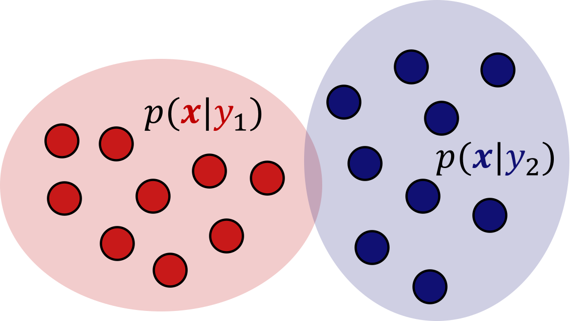
Generative classification
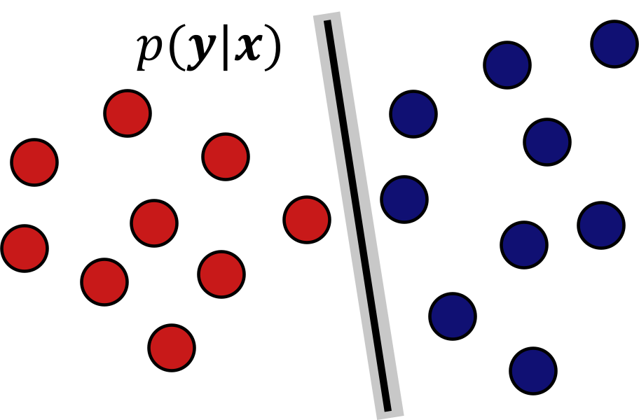
Discriminative classification
Parameter estimation and uncertainty
Discriminative modeling omits the choice of intermediate densities needed for generative classification, yet it still leaves open how the parameters are to be determined. Hence the question remains, how can we obtain the optimal parameters? Again, through Bayesian inference as
\begin{equation}\label{eq:bayes2} p(\mathbf{\theta} \mid \mathbf{x}, \mathbf{y}) = \frac{p(\mathbf{y} \mid \mathbf{x}, \mathbf{\theta}) \,p(\mathbf{\theta})}{p(\mathbf{y} \mid \mathbf{x})}, \end{equation}where independence of $\mathbf{x}$ from $\mathbf{\theta}$ is assumed, $p(\mathbf{\theta})$ represents the prior belief on the parameter distribution, and $p(\mathbf{y}\mid\mathbf{x})$ the conditional data likelihood (i.e., the evidence). After obtaining a posterior with dataset $\mathcal{D}=\{\mathbf{x}_i, \mathbf{y}_i\}_{i=1}^N$, the predictive distribution for a new datapoint $\mathbf{x}^*$ can be denoted as
\begin{equation}\label{eq:predicitve} p(\mathbf{y}\mid \mathbf{x}^*, \mathcal{D})=\int \underbrace{p(\mathbf{y}\mid \mathbf{x}^*,\mathbf{\theta})}_{\text{Data}}\, \overbrace{p(\mathbf{\theta}\mid \mathcal{D})}^{\text{Model}} \mathrm{d}\mathbf{\theta}. \end{equation}As evident, both the variability in the empirical data and the inferred parameters of the model influence the predictive distribution. Given this, a straightforward approach to quantify the total uncertainty is achieved by obtaining the predictive entropy, $H[\,\mathbf{y}\mid\mathbf{x}^*,\mathcal{D}\,]$, i.e. the entropy of the predictive distribution $p(\mathbf{y}\mid \mathbf{x}^*, \mathcal{D})$, as
\begin{equation}\label{eq:uncdec} H[\,\mathbf{y}\mid\mathbf{x}^*,\mathcal{D}\,]= \overbrace{I[\mathbf{y},\mathbf{\theta} \mid \mathbf{x}^*,\mathcal{D}]}^{\text{epistemic}} + \underbrace{\mathbb{E}_{p(\mathbf{\theta}\mid\mathcal{D})}[\,H[\mathbf{y}\mid\mathbf{x}^*,\mathbf{\theta}]\,]}_{\text{aleatoric}}, \end{equation}where $I$ represents the mutual information. The first term is the expected information gain about the parameters $\mathbf{\theta}$ from observing the true label $\mathbf{y}$. A high value reflects epistemic uncertainty, where the model is uncertain enough that the true label would carry substantial information. The second term, the inherent randomness in the data, is obtained by averaging the predictive uncertainty over the posterior of plausible models from Equation \ref{eq:bayes2}. It is the irreducible noise that no amount of additional training data can remove, known as the aleatoric uncertainty.
Nonetheless, determining the nature of uncertainty is rarely straightforward. For example, Hüllermeier and Waegeman2 stated that “by allowing the learner to change the setting, the distinction between these two types of uncertainty will be somewhat blurred”. This sentiment is also shared by Kiureghian and Ditlevsen3, noting that “in one model an addressed uncertainty may be aleatory, in another model it may be epistemic”. Sharing similar views, we highlight the necessity of careful analyses and possible subjective interpretation regarding the topic as we treat the realm of quantifying uncertainty. Especially with increasingly complex methodologies, treating the uncertainties as separate concepts is mostly theoretical (often even more philosophical) and highly non-trivial in practice.
Maximum Likelihood Estimation
Equation \ref{eq:bayes2} still contains the difficult denominator term, i.e. the evidence \( p(\mathbf{y} \mid \mathbf{x}) \). This value can be determined through marginalization over the parameters through
\begin{equation} p(\mathbf{y} \mid \mathbf{x}) = \int p(\mathbf{y} \mid \mathbf{x}, \mathbf{\theta}) p(\mathbf{\theta}) \, \mathrm{d}\mathbf{\theta},\label{eq:intract} \end{equation}but can quickly become computationally infeasible with increasing number of model parameters. Since the likelihoods are in our ultimate interest, it can make sense to simply maximize \( p(\mathbf{y} \mid \mathbf{x}, \mathbf{\theta}) \) directly with Maximum Likelihood Estimation (MLE) as
\begin{equation}\label{eq:mle} \operatorname{MLE} = \arg\max_{\mathbf{\theta}} \, \mathbb{E}_{ P_{\mathbf{Y} \mid \mathbf{X}}} \left[ \log p(\mathbf{y} \mid \mathbf{x}, \mathbf{\theta}) \right], \end{equation}completely omitting the infeasible integral in Equation \ref{eq:intract}. To model $p(\mathbf{y}\mid\mathbf{x}, \mathbf{\theta})$, one can make use of a function $f_{\mathbf{\theta}}:\mathbb{R}^{D}\rightarrow\mathbb{R}^{K}$ that infers the parameters of a PMF as
\begin{equation}\label{eq:modelikelihood} p(\mathbf{y}=k\,\mid\,\mathbf{x}^*,\mathbf{\theta})=\frac{e^{\mathbf{a}_k}}{\sum_j e^{\mathbf{a}_j}}, \end{equation}with channel-wise indexing over the denominator. Furthermore, it is also possible to incorporate prior knowledge on the parameter distribution, using Maximum a Posteriori (MAP) estimations, which is denoted as
\begin{equation} \operatorname{MAP} = \arg\max_{\mathbf{\theta}} \, \mathbb{E}_{P_{\mathbf{Y} \mid \mathbf{X}}} \left[ \log p(\mathbf{y} \mid \mathbf{x}, \mathbf{\theta}) + \log p(\mathbf{\theta}) \right]. \end{equation}This can already be enforced with regularization on the parameters. Penalizing the L1-norm of the weights corresponds to a Laplacian prior, and L2-regularization to a Gaussian one. This connects back to the frequentist versus Bayesian discussion. A frequentist practitioner adding a regularizer assumes no distribution, yet each penalty pairs with a prior that yields the same estimate, so the commitment enters through the choice of penalty rather than a stated belief. MLE is also likely more familiar than it first appears. Standard softmax activated networks normalize their outputs into a distribution over classes, and training maximizes the probability assigned to the correct class index.
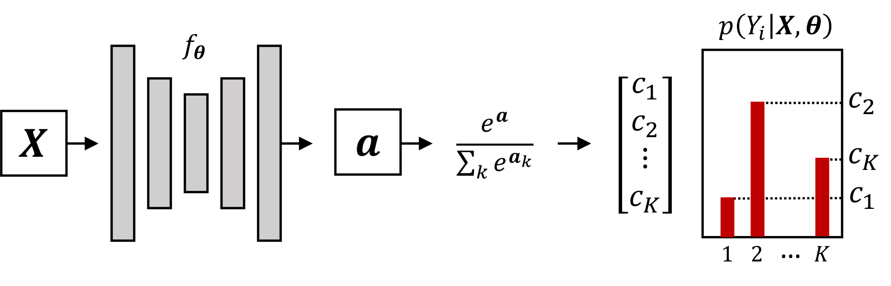
Uncertainty modeling by treating confidence values as parameters of a PMF (no transparency on the SoftMax because I was lazy…).
The KL divergence
In parametric estimation, a family of distributions $\mathcal{P} = \{ p_{\mathbf{\theta}} \mid \mathbf{\theta} \in \Theta \}$ is selected to model the conditional densities, and it is sought to find the parameter $\mathbf{\theta}$ that best approximates $P_{\mathbf{Y}\mid\mathbf{X}}$. We can show that performing MLE is equivalent to minimizing the Kullback-Leibler (KL) divergence (or relative entropy) \begin{subequations}
\begin{align} D_{\text{KL}} [ P_{\mathbf{Y} \mid \mathbf{X}} \, \parallel \, p_{\mathbf{Y} \mid \mathbf{X}}^{\mathbf{\theta}} ] &= \int \log \frac{P(\mathbf{y} \mid \mathbf{x})}{p(\mathbf{y} \mid \mathbf{x}, \mathbf{\theta})} P(\mathbf{y} \mid \mathbf{x}) \, \mathrm{d} \mathbf{y} \\ &= \mathbb{E}_{P_{\mathbf{Y} \mid \mathbf{X}}} \left[ \log \frac{P(\mathbf{y} \mid \mathbf{x})}{p(\mathbf{y} \mid \mathbf{x}, \mathbf{\theta})} \right] \\ &= \mathbb{E}_{P_{\mathbf{Y} \mid \mathbf{X}}} \left[ \log P(\mathbf{y} \mid \mathbf{x}) - \log p(\mathbf{y} \mid \mathbf{x}, \mathbf{\theta}) \right], \end{align}\end{subequations} describing the information loss induced when approximating the true distribution $P_{\mathbf{Y} \mid \mathbf{X}}$ with $p_{\mathbf{Y} \mid \mathbf{X}}^{\mathbf{\theta}}$. Notably, \( P(\mathbf{y} \mid \mathbf{x}) \) is independent of the parameters and thus constant. Furthermore, MAP corresponds to minimizing the same empirical objective augmented with a regularization term $\frac{1}{N} \log p(\mathbf{\theta})$.
The KL divergence also has crucial properties such as non-negativity, asymmetry ($D_{\text{KL}}[P \parallel Q] \neq D_{\text{KL}}[Q \parallel P]$) and convexity. In particular, the asymmetric property of the KL-divergence results in an interesting design choice. The forward KL, $D_{\text{KL}}[P \parallel Q]$ is mode covering, penalizes $Q$ assigning low probability to an outcome likely under $P$, while the reverse KL, $D_{\text{KL}}[Q \parallel P]$ is mode seeking, and penalizes $Q$ generating samples unlikely under $P$.
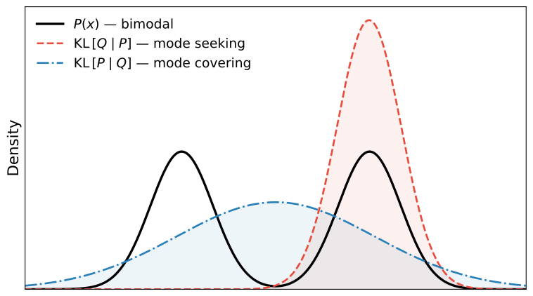
Mode-covering vs. mode-seeking behavior of the forward and reverse KL-divergence, respectively.
Cost trade-offs in generative modeling
The last section showed that MLE can be used to estimate data distributions. In practice it underpins the vast majority of contemporary generative models, which raises the question of in what sense these approaches remain Bayesian at all. Full Bayesian inference requires marginalizing over all uncertain quantities, carrying the prior through the integral as denoted in Equation \ref{eq:predicitve}. Performing this integration, however, is analytically intractable and computationally prohibitive for high-dimensional NNs. Consequently, modern DL accepts two compromises, one over the global parameters and one over the per-datapoint variables. Both replace an integral with an optimization, and both trade a distribution for a point.
The first concerns the parameters. Rather than maintaining a full posterior over them and averaging predictions across it, the parameters are optimized as point estimates. In well-specified regimes with abundant data, the posterior may concentrate sharply around a single region of parameter space, making Bayesian model averaging and point-estimate prediction nearly indistinguishable. In high-dimensional NNs, however, the posterior is typically far more intricate and can remain diffuse along many directions, so collapsing it to a single estimate may systematically understate ambiguity in the parameters. That this collapse generalizes as well as it does, even when explicit priors are weak or absent, is widely attributed to the implicit regularization induced by gradient-based optimization4567, and it is what motivates large training sets, over-parameterization, and powerful optimization heuristics.
The second compromise concerns the per-datapoint variables and is known as amortization, from Old French amortir, ultimately from Latin ad mortem (“to death”). In economics, it refers to the strategy of gradually extinguishing a debt or spreading an asset’s cost over its useful life. ML borrows the concept to describe a computational trade-off. Generative models seek to capture the distribution of the data itself, but high-dimensional observations such as images are far too complex to describe directly. A solution is to assume each observation is generated from a simpler, unobserved quantity, so explaining a datapoint amounts to inferring the quantity that produced it, in principle a separate optimization per input. Amortized inference instead incurs a heavy upfront cost to train a single shared network that maps any input directly to an approximation of the posterior over its unobserved quantity in one forward pass, writing off the need for per-datapoint optimization. The saving is not free. A single shared mapping cannot in general reach what per-datapoint optimization would find, and the residual gap widens on inputs the encoder serves poorly.
Duality of inference
A recurring theme is the fundamental duality between forward problems, predicting effects from known causes, and inverse problems, inferring unknown causes from observed effects. Bayes’ rule in Equation \ref{eq:bayes2} connects these directions by combining the forward model (the likelihood) with a prior to yield the posterior, a probabilistic solution to the inverse problem. In the physical sciences, this mirrors the distinction between two complementary tasks. The forward task uses a system’s governing differential equations, along with its initial and boundary conditions, to simulate its evolution and predict its future state. The inverse task instead works backward from observed trajectories to recover the hidden parameters or conditions that produced them. This inverse direction is often ill-posed and highly sensitive to noise.
In statistical modeling, the same duality is reflected in the nature of the modeled uncertainty. Inverse problems here are typically ill-posed as well, since a linear forward map is blind to anything in its null space, rendering solutions non-unique. Directions with small singular values are transmitted weakly, so inverting amplifies them, and the noise along them dominates the signal. They therefore require strong regularization or prior structure to ensure identifiability and robustness. Forward problems, in contrast, are usually well-posed once a model is specified. Given the causes (inputs and parameters), the mapping to a distribution over predicted effects is defined and can often be evaluated or simulated directly. However, the ambiguity shifts from the cause to which observation is realized, since the predictive distribution may be broad, skewed, or multimodal, as in photon-limited imaging where counts are discrete and highly variable at low intensities.
Interestingly, modern generative models explicitly exploit this bidirectional relationship as well. Through mechanisms such as bijective transformations, variational approximations, adversarial training, and score-based dynamics, they implement the interplay between the forward and reverse directions implied by Bayes’ rule. These frameworks are the subject of the next chapter, which describes how their particular mathematical forms relate simple base noise distributions to coherent, structured data. Taken together, they reveal that the apparent diversity of modern generative modeling rests on a shared foundation of the forward-inverse duality.
Duality of forward and inverse problems in statistics and uncertainty
| Problem | Direction | Statistical Goal (Analysis) | Target uncertainty |
|---|---|---|---|
| Forward | System $\rightarrow$ Data | Given $\tilde{\boldsymbol{\theta}}$, solve $p(\mathbf{X} \mid \tilde{\boldsymbol{\theta}})$ | Noise in $\mathbf{X}$ |
| Inverse | Data $\rightarrow$ System | Given $\tilde{\mathbf{x}}$, analyze $p(\tilde{\mathbf{x}} \mid \boldsymbol{\theta})$ | Ambiguity about $\boldsymbol{\theta}$ |
Closing thoughts
In reality, probabilistic models retain what we typically assume away. Rather than collapsing uncertainty into point estimates, they maintain full distributions over quantities of interest. Of course, treating every variable as a continuous distribution is rarely feasible. As we have shown, a common and practical middle ground is to keep parameters as point estimates while modeling the output as a distribution. However, in our examples so far, we have only learned class-conditional distributions $p(\mathbf{y} \mid \mathbf{x})$. But what if we want to go further and learn the full data distribution $p(\mathbf{x})$ itself? This is a fundamentally harder problem, and tackling it requires introducing latent variables, which are hidden representations that capture the underlying structure of the data. Instead of modeling the observations directly, we learn a compact representation and a mapping from this latent space back to data space. This will be treated in another blog post.
V. Vapnik, The Nature of Statistical Learning Theory, Springer Science & Business Media, 1999 ↩︎
E. Hüllermeier and W. Waegeman, “Aleatoric and epistemic uncertainty in machine learning. An introduction to concepts and methods,” Machine Learning, vol. 110, pp. 457–506, 2021 ↩︎
A. Der Kiureghian and O. Ditlevsen, “Aleatory or epistemic? Does it matter?,” Structural Safety, vol. 31, no. 2, pp. 105–112, 2009 ↩︎
C. Zhang, S. Bengio, M. Hardt, B. Recht, and O. Vinyals, “Understanding deep learning requires rethinking generalization,” ICLR, 2017 ↩︎
B. Neyshabur, R. Tomioka, and N. Srebro, “In search of the real inductive bias. On the role of implicit regularization in deep learning,” ICLR, 2015 ↩︎
S. Gunasekar, B. Woodworth, S. Bhojanapalli, B. Neyshabur, and N. Srebro, “Implicit regularization in matrix factorization,” NeurIPS, 2017 ↩︎
D. Soudry, E. Hoffer, M. S. Nacson, S. Gunasekar, and N. Srebro, “The implicit bias of gradient descent on separable data,” JMLR, vol. 19, pp. 2822–2878, 2018 ↩︎